Evaluating Improper Integrals - AP Calculus BC

SECTION 1

Historical Context & Motivation

The definite integral, as formalized by Newton and Leibniz in the late seventeenth century, was originally conceived for well-behaved functions over bounded, closed intervals. Yet even early practitioners encountered integrals whose domains stretched to infinity or whose integrands blew up at one or more points within the interval of integration. The question of whether such integrals could be assigned finite, meaningful values motivated decades of investigation and ultimately led to the concept of the improper integral. These integrals play a central role in probability, physics, and engineering, where infinite domains and singular behavior are the norm rather than the exception.

1668 • Mercator's Logarithmic Series

Nicholas Mercator published a series expansion of ln(1 + x) involving integration of 1/(1 + x), hinting at the need to handle infinite behavior at the boundary of convergence.

1734 • Euler Evaluates ∫₁∞ dx/x²

Leonhard Euler demonstrated that certain integrals over infinite intervals converge to finite values, laying early groundwork for distinguishing convergent from divergent improper integrals.

1823 • Cauchy's Rigorous Limit Definition

Augustin-Louis Cauchy formalized the improper integral by defining it as the limit of a proper integral, establishing the convergence framework still used in modern calculus courses.

1854 • Riemann's Integral Theory

Bernhard Riemann extended integration theory to characterize integrability conditions, further clarifying when improper integrals can and cannot be evaluated.

The central question that drives this lesson is deceptively simple: when we remove the constraint that an integral must have finite bounds and a bounded integrand, can we still compute a well-defined numerical value? The answer depends entirely on whether a certain limit exists and is finite. Mastering this concept is essential for AP Calculus BC, where improper integrals appear in the context of convergence tests for series, areas under curves extending to infinity, and applications in physics.

SECTION 2

Core Principles & Definitions

An integral is called improper if it fails to satisfy at least one of the two standard requirements for a proper Riemann integral: the interval of integration must be finite, and the integrand must be bounded (i.e., continuous or at least piecewise continuous) on the entire closed interval. When either condition is violated, we cannot directly apply the Fundamental Theorem of Calculus; instead, we express the integral as a limit and determine whether that limit converges to a finite number or diverges.

Type I — Infinite Limits

One or both limits of integration are ±∞. We replace the infinite bound with a variable and take a limit. Example: ∫₁∞ dx/x².

Type II — Discontinuous Integrand

The integrand has an infinite discontinuity at or between the limits. We approach the singularity with a limit. Example: ∫₀¹ dx/√x.

Convergence

An improper integral converges if the defining limit exists and equals a finite number. The integral is then assigned that finite value.

Divergence

An improper integral diverges if the limit does not exist or is ±∞. No finite value can be assigned, and the area is said to be infinite.

Splitting Strategy

When both bounds are infinite or multiple discontinuities exist, split into separate improper integrals. All parts must converge for the whole integral to converge.

✦

KEY TAKEAWAY

Think of evaluating an improper integral like filling an infinitely long trough with water. If the trough narrows quickly enough, the total volume of water (area under the curve) can be finite — the integral converges. If the trough stays wide or narrows too slowly, the water overflows without bound — the integral diverges. The limit operation is the mathematical tool that detects which scenario occurs.

SECTION 3

Visual Explanation: Area Under Curves to Infinity

The shaded cyan region under y = 1/x² from x = 1 to ∞ has finite area equal to 1, illustrating convergence. The dashed red curve y = 1/x also approaches zero, yet its shaded area grows without bound — a classic divergent improper integral. The rate of decay toward zero determines convergence.

The diagram above captures the essential geometric insight behind Type I improper integrals. Both f(x) = 1/x² and g(x) = 1/x are positive and tend to zero as x → ∞, so at first glance, one might expect both to enclose finite areas. The critical difference lies in the rate of decay: 1/x² shrinks fast enough that the cumulative area approaches a horizontal asymptote (the value 1), whereas 1/x decreases so slowly that new area accumulates without bound. This geometric observation is made precise by the p-integral convergence test, which we will formalize in Section 4.

SECTION 4

Mathematical Framework

Type I: Infinite Limits of Integration

TYPE I — UPPER BOUND INFINITE

∫ₐ∞ f(x) dx = lim (b→∞) ∫ₐᵇ f(x) dx

Replace the infinite upper bound with a finite variable b, evaluate the proper integral, then take the limit as b → ∞. If the limit is finite, the integral converges to that value.

TYPE I — LOWER BOUND INFINITE

∫₋∞ᵇ f(x) dx = lim (a→−∞) ∫ₐᵇ f(x) dx

Analogously, replace the infinite lower bound with a and take the limit as a → −∞.

TYPE I — BOTH BOUNDS INFINITE

∫₋∞∞ f(x) dx = ∫₋∞ᶜ f(x) dx + ∫ᶜ∞ f(x) dx

Split at any convenient finite value c. Both integrals must independently converge for the whole integral to converge. The choice of c does not affect the result.

Type II: Discontinuous Integrands

TYPE II — SINGULARITY AT LOWER BOUND

∫ₐᵇ f(x) dx = lim (t→a⁺) ∫ₜᵇ f(x) dx

When f is unbounded as x → a⁺, replace a with t and take the right-hand limit. If the integrand blows up at b, approach from the left: lim (t→b⁻) ∫ₐᵗ f(x) dx.

The p-Integral Test

p-INTEGRAL CONVERGENCE

∫₁∞ dx/xᵖ converges ⟺ p > 1 (and equals 1/(p − 1))

This benchmark integral is the most frequently tested improper integral on the AP exam. When p = 1 the integral equals ln b → ∞ (diverges). When p > 1, the antiderivative is $x^{1−p}$ /(1−p), whose limit as x → ∞ is 0.

⚠

AP Exam Tip

On the AP Calculus BC exam, you must show the limit notation when evaluating an improper integral. Simply plugging in ∞ for a bound without writing "lim" will result in loss of communication points on free-response questions. Always write: lim (b→∞) [F(b) − F(a)].

SECTION 5

Classification & Comparison Tests

Not every improper integral can be evaluated by finding an antiderivative in closed form. In such cases, the Direct Comparison Test and the Limit Comparison Test allow us to determine convergence or divergence by comparing the integrand to a simpler function whose behavior we already know. These tests mirror the comparison tests for infinite series and share the same logical foundations.

This decision flowchart summarizes the evaluation strategy: identify the type of improper integral, rewrite with proper limit notation, attempt an antiderivative, and—if no closed form exists—fall back on comparison tests to determine convergence or divergence.

Test	Hypotheses	Conclusion
Direct Comparison	0 ≤ f(x) ≤ g(x) for all x ≥ a	If ∫ₐ∞ g(x) dx converges, then ∫ₐ∞ f(x) dx converges. If ∫ₐ∞ f(x) dx diverges, then ∫ₐ∞ g(x) dx diverges.
Limit Comparison	f(x) > 0, g(x) > 0, and lim (x→∞) f(x)/g(x) = L where 0 < L < ∞	∫ₐ∞ f(x) dx and ∫ₐ∞ g(x) dx either both converge or both diverge.

Comparison tests for improper integrals

The comparison tests are especially useful when the integrand involves compositions such as e⁻ˣ², sin(x)/x², or other expressions lacking elementary antiderivatives. In practice, you compare against benchmark functions whose convergence is already established—most commonly the p-integrals ∫₁∞ dx/xᵖ and exponential decay integrals such as ∫₁∞ e⁻ˣ dx.

SECTION 6

Worked Example

Evaluate ∫₁∞ dx/x³

1
Step 1 — Identify the Integral Type

The upper limit of integration is ∞, so this is a Type I improper integral. The integrand f(x) = 1/x³ is continuous on [1, ∞), so there are no Type II issues.
2
Step 2 — Rewrite with Limit Notation

Replace the infinite upper bound with b and write: ∫₁∞ dx/x³ = lim (b→∞) ∫₁ᵇ x⁻³ dx.
3
Step 3 — Find the Antiderivative

Apply the power rule: ∫ x⁻³ dx = x⁻²/(−2) = −1/(2x²) + C.

F(x) = −1/(2x²)
4
Step 4 — Apply the Fundamental Theorem

Evaluate the antiderivative from 1 to b: F(b) − F(1) = −1/(2b²) − (−1/2) = −1/(2b²) + 1/2.
5
Step 5 — Take the Limit

lim (b→∞) [−1/(2b²) + 1/2] = 0 + 1/2 = 1/2. Since the limit is a finite number, the improper integral converges.

∫₁∞ dx/x³ = 1/2

Evaluate ∫₀¹ dx/√x (Type II)

1
Step 1 — Identify the Integral Type

The integrand f(x) = 1/√x = x⁻¹ᐟ² has an infinite discontinuity at x = 0, the lower limit. This is a Type II improper integral.
2
Step 2 — Rewrite with Limit Notation

∫₀¹ dx/√x = lim (t→0⁺) ∫ₜ¹ x⁻¹ᐟ² dx.
3
Step 3 — Find the Antiderivative

∫ x⁻¹ᐟ² dx = x¹ᐟ²/(1/2) = 2√x + C.

F(x) = 2√x
4
Step 4 — Evaluate and Take the Limit

F(1) − F(t) = 2√1 − 2√t = 2 − 2√t. Then lim (t→0⁺) (2 − 2√t) = 2 − 0 = 2. The integral converges.

∫₀¹ dx/√x = 2

SECTION 7

Common Pitfalls & Strategies

Common Pitfall	Why It's Wrong	Correct Approach
Plugging ∞ directly into F(x)	∞ is not a real number. Arithmetic with ∞ is undefined in standard calculus.	Always write lim (b→∞) and evaluate the limit formally.
Ignoring interior discontinuities	If the integrand has a vertical asymptote inside [a, b], the FTC does not apply directly; the result will be incorrect.	Split the integral at the discontinuity and evaluate each piece as a separate improper integral.
Using a single limit for ∫₋∞∞	Writing lim (b→∞) ∫₋ᵇᵇ f(x) dx evaluates the Cauchy Principal Value, which may give a finite answer even when the integral diverges.	Split into two independent limits: lim (a→−∞) and lim (b→∞). Both must converge independently.
Concluding convergence because f(x)→0	f(x)→0 is necessary but not sufficient for ∫ₐ∞ f(x) dx to converge (e.g., 1/x → 0 but ∫₁∞ dx/x = ∞).	Use the p-test, comparison test, or direct evaluation to confirm convergence.

Frequent errors on AP Calculus BC improper integral problems

✦

KEY TAKEAWAY

Improper integrals are like stress-testing a bridge: you do not simply assume it can support infinite traffic—you gradually increase the load (the upper limit b or approach to the singularity) and observe whether the structure (the integral value) stabilizes at a finite capacity or collapses toward infinity. The limit is the mathematical load test.

SECTION 8

Connection to Series & Advanced Theory

Improper integrals and infinite series are deeply intertwined through the Integral Test for series convergence, one of the most powerful tools in AP Calculus BC. If f is a continuous, positive, decreasing function for x ≥ 1 with f(n) = aₙ, then ∑ aₙ from n = 1 to ∞ converges if and only if ∫₁∞ f(x) dx converges. This connection means that your skill in evaluating improper integrals directly transfers to determining whether series converge. For instance, the divergence of ∫₁∞ dx/x immediately implies that the harmonic series ∑ 1/n diverges, while the convergence of ∫₁∞ dx/x² confirms that ∑ 1/n² converges.

Concept	Improper Integrals (This Lesson)	Infinite Series (Advanced)
Object being summed	Continuous function f(x) over [a, ∞)	Discrete sequence aₙ summed from n = 1 to ∞
Convergence mechanism	lim (b→∞) ∫ₐᵇ f(x) dx is finite	lim (N→∞) Sₙ = lim (N→∞) ∑ aₖ from k=1 to N is finite
p-test threshold	∫₁∞ dx/xᵖ converges for p > 1	∑ 1/nᵖ converges for p > 1 (p-series test)
Comparison tests	Direct & Limit Comparison for integrals	Direct & Limit Comparison for series

Parallel structure between improper integrals and infinite series

Beyond the AP curriculum, improper integrals form the backbone of the Laplace transform used in differential equations and control engineering, probability density functions in statistics (where ∫₋∞∞ f(x) dx = 1 by definition), and the Gamma function Γ(n) = ∫₀∞ xⁿ⁻¹ e⁻ˣ dx, which generalizes the factorial. Mastering the evaluation techniques in this lesson prepares you for all of these applications.

SECTION 9

Practice Problems

Question 1: CONCEPTUAL

Which of the following integrals is improper?

A. ∫₀¹ x² dx
B. ∫₁² (1/x) dx
C. ∫₀¹ (1/x²) dx
D. ∫₋₁¹ eˣ dx
E. ∫₀π sin(x) dx

Show answer (C)

The correct answer is C. The integrand 1/x² has an infinite discontinuity at x = 0, the lower limit of integration, making this a Type II improper integral. Option A is a polynomial on a closed interval — perfectly proper. Option B involves 1/x on [1, 2], where the function is continuous and bounded (no singularity since x ≠ 0 on this interval). Option D involves eˣ, which is continuous everywhere, on a finite interval. Option E involves sin(x) on [0, π], also continuous and bounded. Only option C has an integrand that is unbounded at an endpoint of the integration interval.

Question 2: BASIC CALCULATION

Evaluate ∫₁∞ dx/x⁴.

A. 1/4
B. 1/3
C. 1/2
D. 3
E. The integral diverges.

Show answer (B)

The correct answer is B. Write ∫₁∞ x⁻⁴ dx = lim (b→∞) ∫₁ᵇ x⁻⁴ dx. The antiderivative is x⁻³/(−3) = −1/(3x³). Evaluating: lim (b→∞) [−1/(3b³) − (−1/3)] = lim (b→∞) [−1/(3b³) + 1/3] = 0 + 1/3 = 1/3. This is a p-integral with p = 4 > 1, confirming convergence. Option A (1/4) results from incorrectly using p − 1 = 4 − 1 = 3 in the denominator but then miscomputing. Option C (1/2) is the value of ∫₁∞ dx/x³, not x⁴. Option D (3) inverts the fraction incorrectly. Option E is wrong because p = 4 > 1 guarantees convergence.

Question 3: INTERMEDIATE

Determine whether ∫₁∞ dx/(x² + 1) converges or diverges, and if it converges, find its value.

A. Converges to π/4
B. Converges to π/2
C. Converges to arctan(2)
D. Diverges to ∞
E. Converges to 1

Show answer (A)

The correct answer is A. The antiderivative of 1/(x² + 1) is arctan(x). So ∫₁∞ dx/(x² + 1) = lim (b→∞) [arctan(b) − arctan(1)] = π/2 − π/4 = π/4. The integral converges because arctan has a horizontal asymptote at π/2. Option B (π/2) would be the value of ∫₀∞ dx/(x² + 1), not starting from 1. Option C (arctan(2)) is incorrect; this would be the upper bound if we evaluated ∫₀² dx/(x² + 1), not the improper integral from 1 to ∞. Option D is wrong because 1/(x² + 1) ≤ 1/x² for x ≥ 1, and the comparison test confirms convergence. Option E (1) is simply incorrect.

Question 4: APPLIED

5 pts

In a physics model, the gravitational potential energy of a satellite launched radially outward from Earth's surface (radius R) is modeled by the integral W = ∫ᵣ∞ (GMm/r²) dr, where G, M, and m are positive constants. (a) Classify this integral and explain why it is improper. (1 point) (b) Use proper limit notation to set up the evaluation. (1 point) (c) Find the antiderivative and evaluate the limit. (2 points) (d) Interpret your result: what does the finite value of this integral mean physically? (1 point)

Show answer

Point-by-point rubric: (a) [1 point] This is a Type I improper integral because the upper limit of integration is ∞. The integrand GMm/r² is continuous for r ≥ R > 0, so the only issue is the infinite bound. (b) [1 point] W = lim (b→∞) ∫ᵣᵇ (GMm/r²) dr. The student must explicitly write the limit notation with a finite upper bound b replacing ∞. (c) [2 points — 1 for antiderivative, 1 for limit evaluation] The antiderivative of GMm/r² = GMm · r⁻² is GMm · (−r⁻¹) = −GMm/r. Evaluating: lim (b→∞) [−GMm/b − (−GMm/R)] = lim (b→∞) [−GMm/b + GMm/R] = 0 + GMm/R = GMm/R. (d) [1 point] The finite value W = GMm/R represents the total work needed to move the satellite from the surface to infinitely far away — the escape energy. Because this integral converges, only a finite amount of energy is required to escape Earth's gravity, which is why escape velocity is a well-defined, finite quantity. Inverse-square force versus distance, with work from R to 4R and the remaining tail toward infinity. Total work is GMm/R.

Inverse-square force versus distance, with work from R to 4R and the remaining tail toward infinity. Total work is GMm/R.

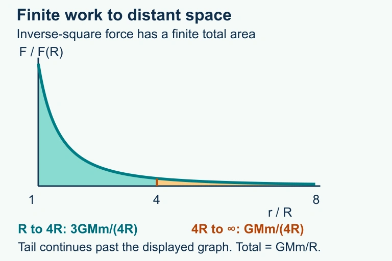Inverse-square gravity requires finite positive work GMm/R to reach arbitrarily distant space, with potential energy referenced separately.

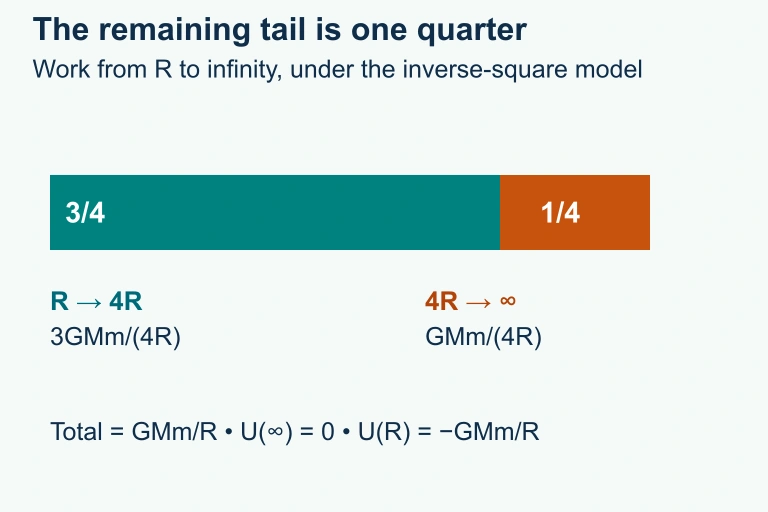The finite work from R to 4R is three quarters of GMm/R; the remaining work to infinity is one quarter. Potential is −GMm/R at R and zero at infinity.

Question 5: CRITICAL THINKING

3 pts

Consider the integral ∫₀∞ dx/(

x^{1/3}

(1 + x)). (a) Explain why this integral has two sources of impropriety. (1 point) (b) Describe how you would split the integral and which comparison functions you would use to argue convergence for each part. You do not need to compute the exact value. (2 points)

Show answer

Point-by-point rubric: (a) [1 point] The integral is improper for two reasons: the integrand 1/(

x^{1/3}

(1 + x)) has an infinite discontinuity at x = 0 (Type II, since

x^{1/3}

→ 0 makes the integrand → ∞), and the upper limit is ∞ (Type I). Both sources must be identified. (b) [2 points — 1 for splitting correctly, 1 for valid comparison functions] Split the integral at a convenient point, say x = 1: ∫₀¹ dx/(

x^{1/3}

(1 + x)) + ∫₁∞ dx/(

x^{1/3}

(1 + x)). For the first piece (near 0): on (0, 1], 1/(1 + x) is bounded between 1/2 and 1, so the integrand behaves like 1/

x^{1/3}

x^{−1/3}

. Since ∫₀¹

x^{−1/3}

dx is a convergent p-integral at 0 (the exponent 1/3 < 1), the first piece converges by Direct Comparison. For the second piece (near ∞): for large x,

x^{1/3}

(1 + x) ≈

x^{1/3}

· x =

x^{4/3}

, so the integrand behaves like 1/

x^{4/3}

. Since ∫₁∞ dx/

x^{4/3}

converges (p = 4/3 > 1), the Limit Comparison Test with g(x) = 1/

x^{4/3}

confirms convergence. Since both pieces converge, the original integral converges.

SUMMARY

Lesson Summary

Summary

An improper integral arises when the interval of integration is infinite (Type I) or when the integrand has an infinite discontinuity (Type II). In every case, the strategy is the same: replace the problematic bound or singularity with a variable, evaluate the resulting proper integral, and take the limit. If the limit is a finite number, the integral converges to that value; otherwise it diverges.

The p-integral test (∫₁∞ dx/xᵖ converges if and only if p > 1) serves as the primary benchmark. When a closed-form antiderivative is unavailable, the Direct Comparison Test and Limit Comparison Test allow you to determine convergence by comparing to known benchmarks. These techniques also provide the foundation for the Integral Test for series, connecting improper integrals to one of the central topics in AP Calculus BC. Always remember: show proper limit notation in every step, split when needed, and never assume convergence without proof.