Volume with Disc Method: Revolving Around Other Axes - AP Calculus BC

SECTION 1

Historical Context & Motivation

The problem of computing volumes of curved solids stretches back to antiquity. Archimedes pioneered the method of exhaustion to calculate the volume of a sphere, essentially summing an infinite collection of thin circular slices—a technique remarkably close to what we now call the disc method. For nearly two millennia, mathematicians lacked a systematic framework for handling arbitrary axes of revolution. The development of integral calculus in the seventeenth century finally provided the algebraic machinery to generalize these ideas, allowing volumes of revolution about any line—not merely the coordinate axes—to be expressed as definite integrals.

~250 BCE • Archimedes' Method of Exhaustion

Archimedes computed the volume of a sphere by summing thin circular cross-sections, prefiguring the disc method by nearly two thousand years.

1615 • Kepler's Nova Stereometria

Johannes Kepler extended the slicing idea to wine barrels and other solids of revolution, computing volumes for practical commerce.

1635 • Cavalieri's Principle

Bonaventura Cavalieri formalized the idea that solids with equal cross-sectional areas at every height have equal volumes, providing a rigorous foundation for the slicing approach.

1666–1687 • Newton & Leibniz Invent Calculus

The fundamental theorem of calculus unified the limit-based slicing process into definite integrals, enabling volumes of revolution about arbitrary axes to be computed systematically.

With calculus in hand, a natural question arises: what happens when the axis of revolution is not the x-axis or y-axis, but some other horizontal or vertical line such as y = 3 or x = −1? The radius of each disc changes, and the formula must be adapted accordingly. This lesson develops the precise adjustments required and shows how the fundamental structure of the disc integral remains intact.

SECTION 2

Core Principles & Definitions

Before tackling non-standard axes, it is essential to solidify the geometric idea underlying every disc-method problem. When a region in the plane is revolved about a line, each thin slice perpendicular to the axis of revolution sweeps out a disc—a flat cylinder whose volume equals π × (radius)² × (thickness). The total volume of the solid is the integral of these infinitesimal disc volumes. The critical step in every problem is correctly identifying the radius of each disc as the distance from the curve to the axis of revolution—not to the coordinate axis.

Axis of Revolution

The fixed line about which the region rotates. It can be any horizontal line y = k or vertical line x = k, not just the coordinate axes.

Disc Radius = Distance to Axis

For revolution about y = k, the radius is |f(x) − k|. For revolution about x = k, the radius is |g(y) − k|. This signed distance is the single most important quantity to identify.

Direction of Integration

Integrate along the axis of revolution: dx for horizontal axes, dy for vertical axes. Limits of integration are determined by the region's projection onto that axis.

No Hole ⇒ Disc (Not Washer)

The disc method applies when every cross-section is a solid circle—no gap between the curve and the axis. If a gap exists, the washer method is needed instead.

✦

KEY TAKEAWAY

Think of each disc as a coin stacked along the axis of revolution. When you shift the axis, you do not change the stacking direction—you change the coin's diameter. An engineer designing a lathe-cut part adjusts the tool's distance from the rotation center, not the spindle itself. Similarly, in the disc formula you adjust the radius expression, not the integral structure.

SECTION 3

Visual Explanation

The diagram below illustrates the key geometric difference between revolving the curve y = √x (from x = 0 to x = 4) about the x-axis versus about the horizontal line y = −1. When the axis shifts downward, every disc's radius grows by 1 unit, fundamentally changing the integrand.

Left: revolving y = √x about the x-axis gives disc radius r = √x. Right: shifting the axis to y = −1 increases the radius to r = √x − (−1) = √x + 1. The dashed lines show each disc's radius measured from the curve to the axis.

Notice that in the left panel the radius of a representative disc at position x is simply √x, measured from the curve down to the x-axis. In the right panel the axis has shifted to y = −1, so the radius extends from the curve at y = √x all the way down to y = −1, giving a radius of √x − (−1) = √x + 1. This single adjustment—replacing f(x) with f(x) − k when the axis is y = k—is the entire conceptual leap required to handle non-standard horizontal axes.

SECTION 4

Mathematical Framework

We now formalize the disc-method integral for revolution about an arbitrary horizontal or vertical line. In every case the structure is the same: V = π ∫ [R(t)]² dt, where R(t) is the distance from the generating curve to the axis, and t is the variable of integration along the direction of the axis.

DISC METHOD — HORIZONTAL AXIS y = k

V = π ∫ₐᵇ [f(x) − k]² dx

f(x) is the curve bounding the region, k is the y-value of the axis of revolution, and [a, b] is the interval on the x-axis over which the region extends. The integrand [f(x) − k]² gives the squared radius of each disc.

DISC METHOD — VERTICAL AXIS x = k

V = π ∫_c^d [g(y) − k]² dy

g(y) is the curve expressed as a function of y, k is the x-value of the vertical axis, and [c, d] is the interval on the y-axis. The disc radius is |g(y) − k|; squaring eliminates the absolute value.

⚠

Sign Convention

Because the radius is squared, the sign of f(x) − k does not matter algebraically—the integral produces the correct positive volume regardless of whether the curve lies above or below the axis. However, when setting up the integral it is wise to verify that the expression inside the square represents a genuine geometric distance. Drawing a representative disc and labeling its radius is the single best safeguard against sign errors on the AP exam.

GENERAL STRATEGY

R(t) = |curve position − axis position|

This single formula covers every disc problem. Identify the curve's coordinate perpendicular to the axis, subtract the axis's coordinate in that same direction, and square the result to build the integrand.

It is worth noting how these formulas reduce to the familiar special cases. When the axis is the x-axis (k = 0), the horizontal formula becomes V = π ∫ₐᵇ [f(x)]² dx, the standard result from most textbooks. When the axis is a line such as y = 5, the radius becomes |f(x) − 5|, and the integrand expands to [f(x) − 5]². Recognizing this pattern prevents the common error of simply plugging f(x) into the integrand without accounting for the shifted axis.

SECTION 5

Detailed Breakdown by Axis Position

The relationship between the axis of revolution and the region determines the disc radius expression. Four common configurations arise on the AP exam, distinguished by whether the axis is above, below, to the left, or to the right of the region. The table below summarizes each case for a region bounded by a single curve and a coordinate axis.

Axis of Revolution	Axis Relative to Region	Disc Radius R	Integral Setup
y = k (k < 0, axis below region)	Below	f(x) − k	V = π ∫ₐᵇ [f(x) − k]² dx
y = k (k > f(x), axis above region)	Above	k − f(x)	V = π ∫ₐᵇ [k − f(x)]² dx
x = k (k < 0, axis left of region)	Left	g(y) − k	V = π ∫_c^d [g(y) − k]² dy
x = k (k > g(y), axis right of region)	Right	k − g(y)	V = π ∫_c^d [k − g(y)]² dy

Four standard configurations for the disc method about non-standard axes

The shaded region between the curve x = y²/3 and x = 5 is revolved about the vertical line x = 5 (pink dashed line). The gold dashed segment at y = 2 shows the disc radius R = 5 − g(y), measured from the curve rightward to the axis.

In the diagram above, because the axis x = 5 lies to the right of the curve x = g(y), the disc radius at height y is R(y) = 5 − g(y). Squaring and integrating with respect to y yields the volume. This "axis to the right" configuration is one of the most commonly tested setups on the AP Calculus BC free-response section, and students should practice sketching the representative disc before writing the integral.

SECTION 6

Worked Example

Let us compute the volume of the solid generated by revolving the region bounded by y = x², y = 0, and x = 2 about the line y = −1.

Volume of Revolution about y = −1

1
Step 1 — Sketch and Identify the Region

The region lies in the first quadrant, bounded above by y = x², below by the x-axis (y = 0), on the left by x = 0 (the y-axis), and on the right by x = 2. The axis of revolution y = −1 is a horizontal line one unit below the x-axis.
2
Step 2 — Determine the Disc Radius

A representative disc at position x has its outer edge on the curve y = x² and extends down to the axis y = −1. The radius is therefore R(x) = x² − (−1) = x² + 1.

R(x) = x² + 1
3
Step 3 — Check for Washer vs. Disc

The region between the x-axis and y = −1 is not part of the bounded region, so this is actually a washer problem! The inner radius is the distance from y = 0 to y = −1, which is r(x) = 0 − (−1) = 1. We need V = π ∫₀² [(x² + 1)² − (1)²] dx.

Note: the gap between y = 0 and y = −1 creates an inner radius.
4
Step 3 (Revised) — Pure Disc Setup

To illustrate a pure disc problem instead, let us change the region: revolve the region bounded by y = x² and the line y = −1 (with x from 0 to 2) directly—that is, the region between the curve and the axis itself. Now every cross-section perpendicular to the x-axis is a complete disc with no hole. The radius is R(x) = x² − (−1) = x² + 1, and we integrate V = π ∫₀² (x² + 1)² dx.

V = π ∫₀² (x² + 1)² dx
5
Step 4 — Expand the Integrand

(x² + 1)² = x⁴ + 2x² + 1. Therefore V = π ∫₀² (x⁴ + 2x² + 1) dx.

Integrand: x⁴ + 2x² + 1
6
Step 5 — Integrate Term by Term

∫₀² (x⁴ + 2x² + 1) dx = [x⁵/5 + 2x³/3 + x] evaluated from 0 to 2. At x = 2: 32/5 + 16/3 + 2 = 32/5 + 16/3 + 2. Finding a common denominator of 15: 96/15 + 80/15 + 30/15 = 206/15.

∫₀² (x⁴ + 2x² + 1) dx = 206/15
7
Step 6 — Multiply by π

V = π × 206/15 = 206π/15 ≈ 43.14 cubic units.

V = 206π/15

💡

Exam Tip

Step 3 above illustrates a critical checkpoint: always verify that the region touches the axis of revolution. If a gap exists between the region and the axis, you have a washer problem, not a disc problem. Misidentifying the cross-section type is one of the most common errors on the AP exam.

A hollow wooden bowl on a stationary lathe accompanies a calibrated generating region and a separate annular cross-section. For 0 ≤ x ≤ 2, rotate the region from y = −1 to y = x² about y = −1. Each full disk has radius x² + 1, so V = π∫₀²(x² + 1)² dx = 206π/15.

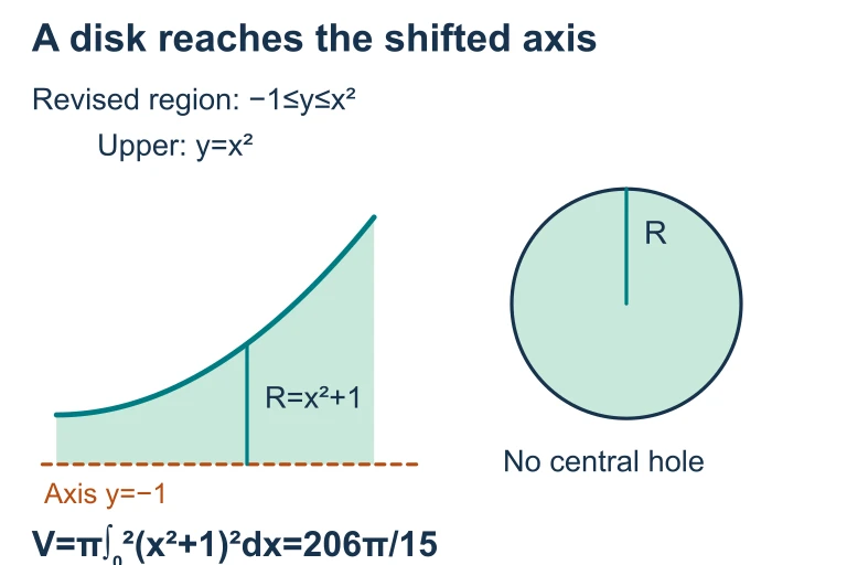For 0 ≤ x ≤ 2, rotate the region from y = −1 to y = x² about y = −1. Each full disk has radius x² + 1, so V = π∫₀²(x² + 1)² dx = 206π/15.

SECTION 7

Disc Method vs. Other Approaches

The disc method is one of several techniques for computing volumes of solids of revolution. Understanding when to deploy it—as opposed to the washer method or the shell method—is essential for efficiency on the AP exam. Below we compare the three approaches, particularly in the context of non-standard axes.

Feature	Disc Method	Washer Method	Shell Method
Cross-section shape	Solid circle (no hole)	Annulus (ring with hole)	Thin cylindrical shell
Integration variable	Along the axis of revolution	Along the axis of revolution	Perpendicular to the axis of revolution
When to use	Region touches the axis; single curve bounds region	Gap between region and axis; two curves bound region	Solving for the other variable is difficult; vertical axis with dx preferred
Radius for y = k axis	\|f(x) − k\|	Outer: \|f(x) − k\|, Inner: \|g(x) − k\|	Shell radius: \|x − h\| (not applicable—uses x = h axis)
Common pitfall	Using disc when a washer is needed (missing inner radius)	Subtracting radii instead of squaring separately	Forgetting the 2π factor

Comparison of volume-of-revolution techniques

🔧

CHOOSING YOUR TOOL

Think of the disc, washer, and shell methods as different lenses on the same 3D solid. The disc method is the simplest lens—one radius, no subtraction—but it only applies when the region directly touches the axis of revolution. If there is a gap, switch to washers. If the algebra of solving for the integration variable is painful, switch to shells. Mastering all three methods and quickly diagnosing which applies is a hallmark of a high-scoring AP student.

SECTION 8

Connection to Advanced Theory

The disc method for non-standard axes connects naturally to more advanced ideas in calculus and beyond. On the AP Calculus BC exam itself, this technique feeds directly into problems involving the washer method (where two radius expressions are subtracted) and parametric or polar volume calculations. In multivariable calculus, the concept generalizes through Pappus's theorem and triple integrals with cylindrical or spherical coordinates.

This Lesson	Advanced Extension
Disc/washer about y = k or x = k	Pappus's centroid theorem: V = 2π × (distance from centroid to axis) × (area of region)
Integration along one variable	Double/triple integrals in cylindrical coordinates: V = ∫∫∫ r dr dθ dz
Revolution of y = f(x)	Revolution of parametric curves: V = π ∫ₐᵇ [y(t)]² x′(t) dt (with sign adjustments for axis shifts)
Known cross-section perpendicular to axis	General cross-section method: A(x) can be any shape (squares, semicircles, equilateral triangles)

From disc method to advanced volume techniques

One particularly elegant connection is Pappus's centroid theorem, which states that the volume of a solid of revolution equals 2π times the distance from the region's centroid to the axis, times the area of the region. This theorem provides a powerful shortcut when the centroid is known, and it also confirms disc/washer results: if you compute the volume by integration and independently by Pappus's theorem, the answers must agree. This cross-check is invaluable in both exam and engineering contexts.

SECTION 9

Practice Problems

Question 1: CONCEPTUAL

The region bounded by y = x and y = 0 from x = 0 to x = 3 is revolved about the line y = −2. Using the washer method, which of the following correctly represents the outer radius R(x) at a general position x?

A. R(x) = x
B. R(x) = x − 2
C. R(x) = x + 2
D. R(x) = 2 − x
E. R(x) = x² + 4

Show answer (C)

The correct answer is C. When revolving about y = −2, we use the washer method because the region (bounded by y = x and y = 0) does not touch the axis of revolution. The outer radius is the distance from the farther curve y = x to the axis y = −2, giving R(x) = x − (−2) = x + 2. Choice A gives only the distance from y = x to the x-axis, ignoring the axis shift. Choice B incorrectly subtracts 2 instead of adding it, which would apply if the axis were y = 2. Choice D yields negative values for x > 2 and represents the wrong geometric direction. Choice E introduces a spurious square and constant that do not correspond to any distance formula.

Question 2: BASIC CALCULATION

Find the volume of the solid generated by revolving the region bounded by y = 3 − √x, y = 0, and x = 0 about the line y = −1.

A. 27π/2
B. 45π/2
C. 54π
D. 63π/2
E. 81π/2

Show answer (D)

The correct answer is D. The curve y = 3 − √x meets y = 0 when 3 − √x = 0, so √x = 3, i.e., x = 9. When revolving about y = −1, the outer radius is the distance from y = −1 to the curve y = 3 − √x, which is R(x) = (3 − √x) − (−1) = 4 − √x. The inner radius is the distance from y = −1 to y = 0, which is r = 0 − (−1) = 1. Using the washer method: V = π∫₀⁹ [(4 − √x)² − 1²] dx = π∫₀⁹ [(16 − 8√x + x) − 1] dx = π∫₀⁹ (15 − 8√x + x) dx = π[15x − 8·(2/3)

x^{3/2}

+ x²/2]₀⁹ = π[15x − (16/3)

x^{3/2}

+ x²/2]₀⁹ = π[15(9) − (16/3)(27) + 81/2] = π[135 − 144 + 81/2] = π[−9 + 81/2] = π(−18/2 + 81/2) = 63π/2.

Question 3: INTERMEDIATE

The region bounded by x = y² and x = 4 is revolved about the line x = 4. Set up and evaluate the integral for the volume using the disc method.

A. V = 256π/5
B. V = 512π/15
C. V = 128π/5
D. V = 64π/3
E. V = 32π

Show answer (B)

The correct answer is B. The parabola x = y² meets x = 4 at y = ±2. The axis x = 4 is the right boundary of the region, so the region touches the axis and the disc method applies. For a disc at height y, the radius is R(y) = 4 − y². The integral is V = π ∫₋₂² (4 − y²)² dy. By symmetry this equals 2π ∫₀² (4 − y²)² dy. Expanding: (4 − y²)² = 16 − 8y² + y⁴. Integrating: ∫₀² (16 − 8y² + y⁴) dy = [16y − 8y³/3 + y⁵/5]₀² = 32 − 64/3 + 32/5 = (480 − 320 + 96)/15 = 256/15. Multiplying: V = 2π × 256/15 = 512π/15. Choice A results from omitting the factor of 2 from symmetry and making an arithmetic error. Choice C comes from an incorrect expansion. Choices D and E use wrong integrand structures.

Question 4: APPLIED

5 pts

A machinist uses a lathe to create a decorative component by rotating the profile y = 4 − x² (for 0 ≤ x ≤ 2) about the line y = −2. The resulting solid extends from the profile curve down to the axis of revolution, forming a solid with no interior hole. (a) Write the integral expression for the volume of this solid using the disc method. (b) Evaluate the integral exactly. (c) A second component is created by instead revolving the same profile about y = 5. Explain whether the disc method applies to this second solid, and if not, identify the correct method.

Show answer

Point 1 (1 pt): Correct radius expression. The disc radius is R(x) = (4 − x²) − (−2) = 6 − x². Award 1 point for the correct radius. Point 2 (1 pt): Correct integral setup. V = π ∫₀² (6 − x²)² dx. Award 1 point for correct limits, integrand, and the factor of π. Point 3 (2 pts): Correct evaluation. Expand: (6 − x²)² = 36 − 12x² + x⁴. Integrate: ∫₀² (36 − 12x² + x⁴) dx = [36x − 4x³ + x⁵/5]₀² = 72 − 32 + 32/5 = 40 + 32/5 = 232/5. Therefore V = 232π/5. Award 1 point for correct antiderivative, 1 point for correct evaluation and final answer. Point 4 (1 pt): The disc method applies to the second solid, consistent with revolving the profile such that the solid extends from the curve to the axis of revolution y = 5 with no interior hole. The radius is R(x) = 5 − (4 − x²) = 1 + x². Award 1 point for correctly stating that the disc method applies with a valid justification.

Question 5: CRITICAL THINKING

4 pts

Let R be the region in the first quadrant bounded by y = xⁿ (n ≥ 1), y = 0, and x = 1. This region is revolved about the line y = −c where c > 0. (a) Explain why the washer method, rather than the disc method, is required here. Set up and evaluate the integral to derive a general formula for the volume V(n, c). (b) Show that V(n, c) = π(1/(2n+1) + 2c/(n+1)) and interpret each term geometrically.

Show answer

Point 1 (1 pt): Setup and method identification. The region R lies between y = 0 and y = xⁿ in the first quadrant, bounded by x = 1. When revolved about y = −c (where c > 0), the axis lies below the region. Since there is a gap from y = −c to y = 0 (the bottom boundary of R), this is a WASHER problem. The outer radius is R(x) = xⁿ + c (distance from y = xⁿ to y = −c) and the inner radius is r(x) = 0 + c = c (distance from y = 0 to y = −c). So V = π ∫₀¹ [(xⁿ + c)² − c²] dx. Award 1 point for correctly identifying the washer setup with both radii. Point 2 (1 pt): Algebraic simplification. Expand: (xⁿ + c)² − c² = x²ⁿ + 2cxⁿ + c² − c² = x²ⁿ + 2cxⁿ. The c² terms cancel. So V = π ∫₀¹ (x²ⁿ + 2cxⁿ) dx. Award 1 point. Point 3 (1 pt): Evaluation. V = π [x²ⁿ⁺¹/(2n+1) + 2cxⁿ⁺¹/(n+1)]₀¹ = π [1/(2n+1) + 2c/(n+1)]. Award 1 point for the correct final formula V(n, c) = π(1/(2n+1) + 2c/(n+1)). Point 4 (1 pt): Geometric interpretation of each term. The first term π/(2n+1) = π ∫₀¹ x²ⁿ dx is the volume obtained by revolving R about the x-axis itself (the disc method with axis y = 0). The second term 2πc/(n+1) = 2πc ∫₀¹ xⁿ dx = 2πc · A, where A = 1/(n+1) is the area of R. By Pappus's centroid theorem, this term represents the additional volume contribution from shifting the axis of revolution c units farther away (from y = 0 to y = −c). Specifically, the total volume by Pappus is V = 2π · d̄ · A where d̄ is the distance from the centroid of R to y = −c. Decomposing d̄ = ȳ + c gives V = 2πȳA + 2πcA, matching the two terms. Award 1 point for correctly interpreting the component terms geometrically.

SUMMARY

Lesson Summary

Summary

The disc method computes volumes of solids of revolution by integrating π[R(t)]² along the axis of revolution. When the axis is a line y = k or x = k (rather than a coordinate axis), the disc radius becomes |f(x) − k| or |g(y) − k|, respectively. The integral structure remains unchanged—only the radius expression is modified.

A critical first step in every problem is to sketch the region and axis and verify whether the region touches the axis of revolution. If it does not, a washer method (or shell method) must be used instead. Mastering the disc method for non-standard axes is foundational for the AP Calculus BC exam, where free-response questions frequently feature revolution about lines such as y = −1, y = 5, x = 3, or other non-zero constants.