Interpreting the Behavior of Accumulation Functions Involving Area - AP Calculus BC

SECTION 1

Historical Context & Motivation

The idea that a quantity can be understood as the running total of its rate of change is one of the deepest insights in the history of mathematics. Long before formal integration existed, ancient Greek mathematicians such as Archimedes computed areas under parabolas by exhaustion—summing ever-finer slices and observing that a single number emerged in the limit. Centuries later, Newton and Leibniz independently recognized that the process of accumulating area under a curve could itself be viewed as a function—one whose derivative recovers the original curve. This reciprocal relationship, codified in the Fundamental Theorem of Calculus, transforms every continuous function f into a new accumulation function F(x) = ∫ from a to x of f(t) dt, whose behavior—where it increases, decreases, or changes concavity—is completely governed by the integrand f.

~250 BCE • Archimedes and Exhaustion

Archimedes computed the area under a parabolic segment by inscribing triangles of decreasing size, effectively performing the first accumulation of area and anticipating integral calculus by nearly two millennia.

1668 • Barrow's Geometric Lectures

Isaac Barrow, Newton's teacher, demonstrated a geometric version of the inverse relationship between tangent (derivative) and area (integral), laying essential groundwork for the Fundamental Theorem.

1687 • Newton's Principia

Newton used 'fluents' (integrals) and 'fluxions' (derivatives) to model motion, treating accumulated displacement as the running integral of velocity—a direct precursor to the accumulation function concept.

1823 • Cauchy's Rigorous Integral

Augustin-Louis Cauchy provided the first ε-δ definition of the integral as a limit of sums, placing the accumulation function on rigorous analytic footing and enabling formal proofs about its continuity and differentiability.

The central question this lesson addresses is: given a graph or formula for f, how can we deduce the behavior of F(x) = ∫ from a to x of f(t) dt without ever computing the antiderivative explicitly? On the AP Calculus BC exam, you will regularly encounter graphs of f and be asked to determine where F is increasing or decreasing, locate its relative extrema, identify intervals of concavity, and find inflection points—all by reading the sign and behavior of f directly.

SECTION 2

Core Principles & Definitions

An accumulation function is defined as F(x) = ∫ from a to x of f(t) dt, where a is a fixed lower limit and x is the variable upper limit. The Fundamental Theorem of Calculus, Part 1 tells us that F′(x) = f(x) whenever f is continuous, which means the integrand itself acts as the derivative of the accumulation function. This single fact unlocks a cascade of interpretive tools: the first-derivative test applies to f to characterize F, and f′ (the derivative of the integrand) serves as F″, governing the concavity of F.

Accumulation Function

F(x) = ∫ from a to x of f(t) dt gives the net signed area under f from a to x. When f is above the t-axis, area accumulates positively; when f is below, area accumulates negatively.

FTC Part 1: F′(x) = f(x)

The derivative of the accumulation function equals the integrand evaluated at x. This links the sign of f(x) directly to whether F is increasing or decreasing at x.

Increasing / Decreasing

F is increasing where f(x) > 0 (positive area is being added) and decreasing where f(x) < 0 (net area is shrinking). A zero of f is a candidate for a relative extremum of F.

Concavity via f′

Since F″(x) = f′(x), the concavity of F depends on whether f is increasing (F concave up) or decreasing (F concave down). Inflection points of F occur where f has local extrema.

Initial Value F(a) = 0

By definition, F(a) = ∫ from a to a of f(t) dt = 0. This anchoring point is essential when you need to find specific values of F or sketch its graph.

✦

KEY TAKEAWAY

Think of the accumulation function like a bank account whose balance at any time equals the running total of deposits and withdrawals. The integrand f is the rate of cash flow: when f is positive, money flows in and the balance (F) rises; when f is negative, money flows out and the balance drops. The rate at which that cash flow itself is changing (f′) determines whether the balance curve bends upward or downward—just as accelerating income growth makes your savings curve steepen, or decelerating income makes it flatten.

SECTION 3

Visual Explanation — From f to F

The diagram below shows a continuous function f on the interval [0, 8] and the corresponding accumulation function F(x) = ∫ from 0 to x of f(t) dt. Study how the sign and shape of f translate directly into the behavior of F. Regions where f is positive correspond to intervals where F is increasing, while regions where f is negative correspond to intervals where F is decreasing. Where f crosses zero with a sign change, F attains a relative extremum. Where f has a local maximum or minimum (meaning f′ changes sign), F has an inflection point.

Top panel: the integrand f(t) with positive regions shaded green and negative regions shaded red. Bottom panel: the accumulation function F(x). Where f crosses zero, F has a relative extremum (yellow dots). Where f reaches a local extreme (its slope changes sign), F has an inflection point (orange dashed lines).

In the top panel, observe that f is positive on (0, 2) and (4, 6) and negative on (2, 4) and (6, 8). In the bottom panel, F rises on those first intervals and falls on the latter ones—exactly matching the sign of f. The relative maximum of F at x = 2 occurs because f transitions from positive to negative there; the relative minimum of F at x = 4 corresponds to f changing from negative to positive. The inflection points of F, marked by the orange dashed lines, align with the locations where f achieves a local extremum—because at those t-values, f′ changes sign, meaning F″ changes sign.

SECTION 4

Mathematical Framework

The theoretical backbone of accumulation function analysis rests on two pillars: the Fundamental Theorem of Calculus (Part 1) and the standard derivative tests applied through the lens of that theorem. Below are the key equations and the logic that connects them.

ACCUMULATION FUNCTION DEFINITION

F(x) = ∫ₐˣ f(t) dt

Here a is a fixed constant, x is the variable upper limit, and f is assumed continuous on an interval containing a. The dummy variable t distinguishes the integration variable from the limit.

FTC PART 1 — FIRST DERIVATIVE

F′(x) = f(x)

The derivative of F at x equals the integrand evaluated at x. Consequently, F is increasing where f(x) > 0 and decreasing where f(x) < 0. Zeros of f where f changes sign are critical points of F and yield relative extrema by the first-derivative test.

SECOND DERIVATIVE — CONCAVITY

F″(x) = f′(x)

Because F′ = f, differentiating again gives F″ = f′. Therefore F is concave up where f is increasing and concave down where f is decreasing. Points where f has a local maximum or minimum correspond to inflection points of F (provided f′ actually changes sign).

CHAIN RULE EXTENSION

d/dx [∫ₐ^{g(x)} f(t) dt] = f(g(x)) · g′(x)

When the upper limit is a composite function g(x) rather than simply x, the chain rule introduces the factor g′(x). On AP Calculus BC, this extension appears frequently and requires careful attention to the inner derivative.

💡

Exam Tip

When a problem gives you the graph of f and asks about F, translate every question into the language of f. 'Where is F increasing?' becomes 'Where is f positive?' 'Where is F concave up?' becomes 'Where is f increasing?' You never need to compute F explicitly.

A stirred transparent tank has one upper inlet and one lower outlet with a valve. The exact diagram links its 100 L salt balance to a computed approach to equilibrium. Suppose a tank receives and releases 4 gal/min for 5 minutes. Its 200 gal inventory stays constant while 20 gal enters and 20 gal leaves: net change is zero and total throughput is 40 gal.

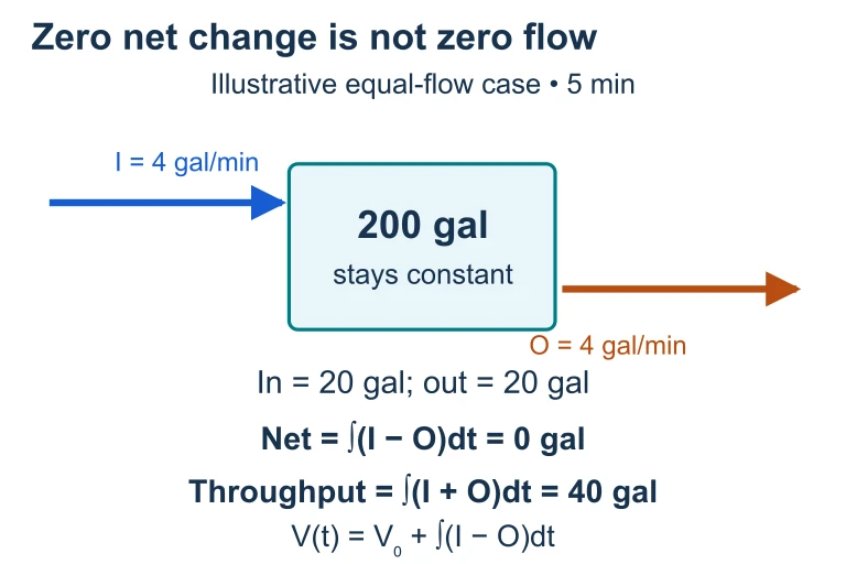Suppose a tank receives and releases 4 gal/min for 5 minutes. Its 200 gal inventory stays constant while 20 gal enters and 20 gal leaves: net change is zero and total throughput is 40 gal.

SECTION 5

Detailed Sign-Chart Breakdown

To systematically interpret an accumulation function, construct a multi-row sign chart that tracks f, f′, and their implications for F. The following table and diagram illustrate how each row of the chart maps onto the behavior of F. This technique is especially valuable on the AP free-response section, where organizing information clearly earns communication points.

Condition on f or f′	Implication for F	Graphical Signature
f(x) > 0	F is increasing (F′ > 0)	F graph rises from left to right
f(x) < 0	F is decreasing (F′ < 0)	F graph falls from left to right
f(x) = 0 with sign change + → −	F has a relative maximum	F reaches a peak
f(x) = 0 with sign change − → +	F has a relative minimum	F reaches a valley
f′(x) > 0 (f increasing)	F is concave up (F″ > 0)	F curves upward (bowl shape)
f′(x) < 0 (f decreasing)	F is concave down (F″ < 0)	F curves downward (cap shape)
f has a local extremum	F has an inflection point	F changes concavity direction

Complete mapping from the integrand f and its derivative f′ to the behavior of the accumulation function F.

A multi-row sign chart showing how the signs of f and f′ determine F's increasing/decreasing behavior, concavity, and extrema. Reading down each column reveals all features of F on that interval.

The sign chart is a powerful organizational tool on exam day. Begin by listing the zeros of f where it changes sign—these are the critical numbers of F. Then determine the sign of f on each sub-interval to fill in F's monotonic behavior. Next, identify where f itself has local extrema (i.e., where f′ changes sign) to locate F's inflection points. Finally, use f's monotonicity on each sub-interval to determine F's concavity. This systematic approach prevents sign errors and ensures you capture every feature the question asks about.

SECTION 6

Worked Example

Consider the function f defined on [0, 6] whose graph consists of line segments connecting the points (0, 4), (2, 0), (4, −2), and (6, 0). Let F(x) = ∫ from 0 to x of f(t) dt. We will determine where F is increasing and decreasing, locate its relative extrema, find its inflection points, and compute F(6).

Full Analysis of F from a Piecewise-Linear f

1
Step 1 — Identify the formula for f on each segment

On [0, 2], f decreases linearly from 4 to 0, so f(t) = 4 − 2t. On [2, 4], f decreases linearly from 0 to −2, so f(t) = −t + 2. On [4, 6], f increases linearly from −2 to 0, so f(t) = t − 6.

f(t) is piecewise linear: {4 − 2t on [0,2]; −t + 2 on [2,4]; t − 6 on [4,6]}
2
Step 2 — Determine where F is increasing and decreasing

Since F′(x) = f(x), we need the sign of f. On (0, 2), f(t) = 4 − 2t > 0 for t < 2, so F is increasing. On (2, 6), f(t) < 0 (the graph is below the t-axis), so F is decreasing on the entire interval (2, 6).

F increasing on (0, 2); F decreasing on (2, 6)
3
Step 3 — Identify relative extrema of F

The only zero of f with a sign change is at x = 2, where f transitions from positive to negative. By the first-derivative test, F has a relative (and absolute) maximum at x = 2. Although f(6) = 0, f does not change sign there on the given domain, so x = 6 is not a relative extremum in the interior.

F has a relative maximum at x = 2
4
Step 4 — Determine concavity and inflection points

F″(x) = f′(x). On (0, 2), f′ = −2 < 0, so F is concave down. On (2, 4), f′ = −1 < 0, so F is still concave down. On (4, 6), f′ = 1 > 0, so F is concave up. Because F″ = f′ changes sign from negative to positive at x = 4, there is an inflection point at x = 4. Note: at x = 2, f has a corner (f′ changes from −2 to −1) but f′ does not change sign—it remains negative—so there is no inflection point there.

F concave down on (0, 4), concave up on (4, 6); inflection point at x = 4
5
Step 5 — Compute F(6) using geometric area

F(6) = ∫₀⁶ f(t) dt, which we compute as the sum of signed areas. On [0, 2]: the triangle has base 2 and height 4, so area = ½ × 2 × 4 = 4 (positive). On [2, 4]: the triangle has base 2 and height 2 (below axis), so signed area = −½ × 2 × 2 = −2. On [4, 6]: the triangle has base 2 and height 2 (below axis), so signed area = −½ × 2 × 2 = −2. Therefore F(6) = 4 − 2 − 2 = 0.

F(6) = 0

ℹ

Why This Matters on the AP Exam

Free-response questions often present the graph of f and define F as its accumulation function. You are expected to justify claims about F using the relationship F′ = f and F″ = f′. Always cite the Fundamental Theorem explicitly—writing 'because F′(x) = f(x) by the FTC' earns justification points in the rubric.

SECTION 7

Common Pitfalls & Strategies

Common Mistake	Why It's Wrong	Correct Approach
Confusing the graph of f with the graph of F	The given graph is the derivative of F, not F itself. Reading it as F leads to wrong extrema and concavity conclusions.	Always remind yourself: the graph you see is F′. Zeros of this graph are critical points of F.
Saying F = 0 wherever f = 0	f(x) = 0 means F′(x) = 0, not F(x) = 0. The value of F at that point depends on the accumulated area up to x.	Compute F at specific points by adding signed areas from the starting point a.
Forgetting the chain rule when the upper limit is g(x)	d/dx [∫ₐ^{g(x)} f(t) dt] = f(g(x)) · g′(x), not just f(g(x)). Omitting g′(x) is a common chain-rule error.	Always check whether the upper limit is a composite function; if so, multiply by the inner derivative.
Claiming inflection point where f has a zero	Inflection points of F occur where F″ = f′ changes sign, i.e., where f has a local extremum—not where f is zero.	For inflection points of F, look at where f changes from increasing to decreasing or vice versa.
Ignoring signed area (treating all area as positive)	The definite integral produces net signed area. Regions below the axis contribute negative values to F.	Carefully track which portions of the graph lie above and below the axis, and assign the correct sign.

Five frequent errors on accumulation function problems and how to avoid them.

✦

KEY TAKEAWAY

An accumulation function problem is fundamentally a derivative-test problem in disguise. The given information (the graph of f) is actually the first derivative of the function you're analyzing (F). Treat every question about F as a question about f: increasing/decreasing comes from the sign of f; concavity comes from whether f is rising or falling. If you internalize this one-level shift, these problems become routine applications of first- and second-derivative tests.

SECTION 8

Connections to Advanced Topics

The accumulation function concept extends naturally to several advanced topics that appear on the AP Calculus BC exam and in subsequent mathematics courses. Understanding these connections deepens your mastery and prepares you for problems that combine accumulation with other integration techniques.

Standard Accumulation	Advanced Extension
F(x) = ∫ₐˣ f(t) dt with constant lower limit	G(x) = ∫_{h(x)}^{g(x)} f(t) dt with variable limits on both ends; differentiate using G′(x) = f(g(x))·g′(x) − f(h(x))·h′(x)
Interpreting net signed area geometrically	Area between curves: ∫ₐᵇ \|f(t) − g(t)\| dt requires careful sign analysis and often splits into sub-intervals
Accumulation of a rate to find a quantity	Differential equations: dy/dx = f(x) with y(a) = y₀ yields y(x) = y₀ + ∫ₐˣ f(t) dt, connecting initial-value problems directly to accumulation
F(x) for continuous f with closed-form area	Accumulation functions defined by integrals with no elementary antiderivative (e.g., erf(x) = (2/√π) ∫₀ˣ $e^{−t²}$ dt), where FTC still governs behavior despite the lack of a formula for F
Single-variable accumulation	In multivariable calculus, line integrals accumulate a function along a curve, and the Fundamental Theorem for Line Integrals is the direct generalization of FTC Part 1

How standard accumulation function analysis connects to more advanced calculus topics.

On the AP Calculus BC exam specifically, accumulation function problems frequently appear alongside particle motion (where position is the integral of velocity), rate-in/rate-out contexts (where total quantity is the integral of a net rate), and improper integrals (where accumulation extends to infinite limits). In each context, the interpretive framework remains the same: the sign of the integrand controls monotonicity, and the behavior of the integrand controls concavity. Mastering this single concept equips you to handle a remarkably wide array of exam questions.

SECTION 9

Practice Problems

Question 1: CONCEPTUAL

Let F(x) = ∫₁ˣ f(t) dt, where f is continuous on [1, 7]. The graph of f is positive and decreasing on (1, 5), crosses zero at x = 5, and is negative on (5, 7). Which of the following statements about F is true?

A. F is increasing on (1, 7) because f is defined everywhere on this interval.
B. F has a relative minimum at x = 5 because f(5) = 0.
C. F has a relative maximum at x = 5 and is concave down on (1, 5).
D. F has an inflection point at x = 5 because f changes sign there.
E. F is concave up on (1, 5) because f is positive there.

Show answer (C)

The correct answer is C. Since F′(x) = f(x) by the FTC, F is increasing where f > 0, i.e., on (1, 5), and decreasing where f < 0, i.e., on (5, 7). At x = 5, f changes from positive to negative, so F has a relative maximum. Because f is decreasing on (1, 5), we have F″(x) = f′(x) < 0 on this interval, meaning F is concave down there. Choice A is wrong because F decreases on (5, 7) where f < 0. Choice B incorrectly identifies a minimum; since f goes from + to −, it's a maximum. Choice D confuses extrema of F with inflection points; a sign change of f produces an extremum of F, not an inflection point. Choice E confuses the sign of f (which controls monotonicity) with the sign of f′ (which controls concavity); f being positive means F is increasing, not concave up.

Question 2: BASIC CALCULATION

Let g(x) = ∫₀ˣ (3t² − 6t) dt. What is g(3)?

A. −9
B. 0
C. 9
D. 18
E. 27

Show answer (B)

The correct answer is B. Compute the antiderivative: ∫(3t² − 6t) dt = t³ − 3t². Evaluating at the bounds: g(3) = [3³ − 3(3²)] − [0³ − 3(0²)] = [27 − 27] − [0] = 0. Choice A (−9) might result from evaluating only −3t² at t = 3. Choice C (9) could come from computing |27 − 27| + 9 incorrectly. Choice D (18) might arise from integrating 3t² alone and getting 27, then subtracting 9 incorrectly. Choice E (27) is the result of integrating only 3t² without the −6t term.

Question 3: INTERMEDIATE

Let F(x) = ∫₀^{x²} sin(t) dt. What is F′(x)?

A. sin(x²)
B. 2x · sin(x²)
C. −cos(x²) + 1
D. 2x · cos(x²)
E. sin(2x)

Show answer (B)

The correct answer is B. By the FTC with the chain rule: d/dx [∫₀^{g(x)} f(t) dt] = f(g(x)) · g′(x). Here f(t) = sin(t) and g(x) = x², so g′(x) = 2x. Therefore F′(x) = sin(x²) · 2x = 2x sin(x²). Choice A forgets the chain rule factor g′(x) = 2x. Choice C computes the antiderivative of sin(t) and evaluates it—this gives F(x), not F′(x). Choice D incorrectly uses cos instead of sin when applying the FTC. Choice E conflates sin(x²) with sin(2x), which are entirely different functions.

Question 4: APPLIED

5 pts

Water flows into a tank at a rate of R(t) = 6 − 2t gallons per minute for 0 ≤ t ≤ 5. The tank initially contains 10 gallons of water. Let W(t) be the number of gallons in the tank at time t. (a) Write an expression for W(t) involving an integral. (b) Find the time at which the tank contains the most water. Justify your answer. (c) How much water is in the tank at t = 5? (d) On what interval is the graph of W concave up? Explain your reasoning.

Show answer

Point 1 (1 pt): W(t) = 10 + ∫₀ᵗ R(s) ds = 10 + ∫₀ᵗ (6 − 2s) ds. Point 2 (1 pt): W′(t) = R(t) = 6 − 2t. Setting W′(t) = 0 gives t = 3. Since R(t) > 0 for t < 3 and R(t) < 0 for t > 3, W is increasing then decreasing. By the first-derivative test, W has an absolute maximum at t = 3. Point 3 (1 pt): W(5) = 10 + ∫₀⁵ (6 − 2t) dt = 10 + [6t − t²]₀⁵ = 10 + (30 − 25) − 0 = 10 + 5 = 15 gallons. Point 4 (1 pt): W″(t) = R′(t) = −2 for all t in (0, 5). Since W″(t) = −2 < 0 everywhere, the graph of W is concave down on the entire interval (0, 5). There is no interval on which W is concave up. Point 5 (1 pt): Correct use of the Fundamental Theorem of Calculus throughout, including the explicit connection W′(t) = R(t) and justification language such as 'by the FTC' or 'since the derivative of the accumulation function equals the integrand.'

Question 5: CRITICAL THINKING

3 pts

Let f be a continuous function on [−3, 3] with f(−3) = 0, and define F(x) = ∫_{−3}^{x} f(t) dt. Suppose that f is strictly increasing on [−3, 0] with f(0) = 2, and strictly decreasing on [0, 3] with f(3) = −1. Also, f(c) = 0 for exactly one value c in (0, 3). (a) Determine all values of x in (−3, 3) where F has a relative extremum, and classify each as a relative maximum or minimum. Justify your answer. (b) Determine all values of x in (−3, 3) where F has an inflection point. Justify your answer.

Show answer

Point 1 (1 pt): By the Fundamental Theorem of Calculus, F′(x) = f(x). Since f(−3) = 0 and f is strictly increasing on [−3, 0], we have f(x) > 0 for all x in (−3, 0]. On (0, 3), f decreases from f(0) = 2 to f(3) = −1, so f(c) = 0 for exactly one c in (0, 3), meaning f is positive on (−3, c) and negative on (c, 3). Since F′(x) = f(x) changes from positive to negative at x = c, F has a relative maximum at x = c by the first-derivative test. There are no other sign changes of f on (−3, 3), so this is the only relative extremum in (−3, 3). Point 2 (1 pt): F″(x) = f′(x). Since f is strictly increasing on (−3, 0), f′(x) > 0 on (−3, 0), so F is concave up on (−3, 0). Since f is strictly decreasing on (0, 3), f′(x) < 0 on (0, 3), so F is concave down on (0, 3). Therefore F″ changes sign at x = 0, so F has an inflection point at x = 0. Point 3 (1 pt): Complete and correct justification: citing F′ = f for extrema analysis and F″ = f′ for concavity analysis, and correctly noting that f has a maximum at x = 0 (since f is increasing then decreasing there), which produces the inflection point of F.

SUMMARY

Lesson Summary

Summary

An accumulation function F(x) = ∫ₐˣ f(t) dt represents the net signed area under the curve f from a to x. By the Fundamental Theorem of Calculus (Part 1), F′(x) = f(x), so the sign of f directly determines where F is increasing or decreasing. Zeros of f where a sign change occurs produce relative extrema of F. Since F″(x) = f′(x), the concavity of F depends on whether f is increasing (concave up) or decreasing (concave down), and inflection points of F occur where f has local extrema.

When the upper limit is a composite function g(x), remember the chain rule extension: d/dx [∫ₐ^{g(x)} f(t) dt] = f(g(x)) · g′(x). For the exam, always build a sign chart tracking f and f′ to systematically extract the full behavior of F, and cite the FTC explicitly in your justifications to earn full rubric credit.