Finding the Area Between Curves Expressed as Functions of y - AP Calculus BC

SECTION 1

Historical Context & Motivation

The idea of computing areas bounded by curves is one of the oldest motivations for what eventually became integral calculus. Ancient Greek mathematicians, most notably Archimedes, devised the method of exhaustion to approximate areas enclosed by parabolas and circles by inscribing sequences of polygons whose areas converged to the desired value. While these early techniques were ingenious, they were limited to specific geometric shapes and lacked a general algebraic framework for handling arbitrary curves. The conceptual leap from vertical slicing—integrating with respect to x—to horizontal slicing with respect to y became natural only after Leibniz and Newton established the formal machinery of the integral in the late seventeenth century, enabling mathematicians to choose the variable of integration that best suits a given geometric configuration.

~250 BCE • Archimedes' Method of Exhaustion

Archimedes computed the area of a parabolic segment by inscribing triangles, effectively performing the first known area-between-curves calculation.

1665–1676 • Newton & Leibniz Develop Calculus

The Fundamental Theorem of Calculus unified differentiation and integration, providing a systematic tool for computing areas under and between curves.

1684 • Leibniz Publishes Integral Notation

Leibniz introduced the ∫ symbol and the differential dy, making it notationally straightforward to integrate with respect to y rather than x.

18th–19th Century • Generalization to Arbitrary Variables

Euler, Cauchy, and Riemann formalized the definite integral with arbitrary limits and variables, solidifying horizontal integration as a standard technique in analysis.

When two curves are more naturally described as functions of y—for instance, a sideways parabola x = y² and a vertical line x = 4—slicing vertically with respect to x would require splitting the region or solving for multiple branches. The central question this lesson addresses is: how can we set up and evaluate a single integral that captures the entire enclosed area by integrating with respect to y?

SECTION 2

Core Principles & Definitions

Before diving into calculations, it is essential to establish the foundational ideas that govern horizontal integration. When we integrate with respect to y, we think of each infinitesimal strip as a horizontal rectangle of width dy and length equal to the horizontal distance between the right curve and the left curve. The following principles outline the framework for setting up such integrals correctly.

Functions of y

Express both bounding curves as x = f(y) and x = g(y). If a curve is given as y = h(x), solve for x in terms of y before proceeding.

Right Minus Left

At each y-value in the interval, the integrand is x_right − x_left, analogous to the 'top minus bottom' principle when integrating with respect to x.

Limits of Integration in y

The lower and upper limits are the y-coordinates where the two curves intersect (or where the region begins and ends vertically).

Absolute Value Guarantee

Because area is always non-negative, ensure x_right ≥ x_left over the entire interval. If the curves cross, split the integral at the crossing y-value.

✦

KEY TAKEAWAY

Think of horizontal integration like measuring the width of a swimming pool at every depth. At each depth y, you measure from the left wall to the right wall; then you add up all those widths multiplied by a tiny depth increment dy. The total gives you the area of the pool's cross-section—just as integrating (x_right − x_left) dy gives you the area of the region between the curves.

SECTION 3

Visual Explanation

The diagram below illustrates the core geometric idea. Two curves, x = f(y) and x = g(y), enclose a region in the xy-plane. Rather than slicing the region into vertical strips (which might require splitting the region or dealing with multi-valued functions), we slice it into horizontal strips of thickness dy. Each strip extends from the left boundary g(y) to the right boundary f(y), so its length is f(y) − g(y). Summing these infinitesimal rectangular areas from y = c to y = d yields the total enclosed area.

The shaded region is bounded on the left by x = g(y) (violet) and on the right by x = f(y) (cyan). A representative horizontal strip at height y has width f(y) − g(y) and thickness dy. The limits of integration run from y = c (bottom intersection) to y = d (top intersection).

SECTION 4

Mathematical Framework

The formal setup for computing the area between two curves expressed as functions of y mirrors the familiar dx-integration formula but with the roles of the axes swapped. Where vertical integration uses "top minus bottom" with respect to x, horizontal integration uses "right minus left" with respect to y. The derivation begins with a Riemann sum of horizontal rectangles and passes to a limit, yielding the definite integral below.

AREA BETWEEN CURVES (FUNCTIONS OF y)

A = ∫ from c to d [f(y) − g(y)] dy

where x = f(y) is the right boundary, x = g(y) is the left boundary, and [c, d] is the interval of y-values over which the region extends.

To derive this, partition the interval [c, d] into n sub-intervals each of width Δy = (d − c)/n. In the i-th sub-interval, choose a sample point y_i*. The area of the i-th horizontal rectangle is [f(y_i*) − g(y_i*)] Δy. Summing and taking the limit as n → ∞ yields the integral.

RIEMANN SUM DERIVATION

A = lim (n→∞) Σ [f(yᵢ*) − g(yᵢ*)] Δy = ∫ from c to d [f(y) − g(y)] dy

This limit exists whenever f and g are continuous on [c, d], which is guaranteed by the Fundamental Theorem of Calculus.

FINDING INTERSECTION POINTS

f(y) = g(y) → solve for y = c and y = d

Set the right-boundary function equal to the left-boundary function. The solutions give the limits of integration.

💡

When to Integrate with Respect to y

Choose dy-integration when: (1) the curves are given as x = f(y) or are easier to solve for x; (2) vertical slicing would require multiple integrals due to the region's shape; or (3) the left/right boundaries change with x but remain consistent as functions of y. If neither variable offers an obvious advantage, try both setups and pick the simpler integral.

SECTION 5

Setting Up Integrals: A Step-by-Step Procedure

To solidify the technique, let us walk through the setup procedure with a concrete geometric example. Consider the region enclosed by the curves x = y² (a rightward-opening parabola) and x = y + 2 (a line). Both curves are already expressed as functions of y, making horizontal integration the natural choice. The diagram below shows the region and the representative horizontal strip.

The parabola x = y² (pink) and the line x = y + 2 (cyan) intersect at (1, −1) and (4, 2). At each y-value in [−1, 2], the line lies to the right of the parabola, so the integrand is (y + 2) − y². The representative horizontal strip (green) illustrates the width and thickness dy.

Step 1 – Express both curves as functions of y. We already have x = y² and x = y + 2.
Step 2 – Find the intersection points. Set y² = y + 2, giving y² − y − 2 = 0, which factors as (y − 2)(y + 1) = 0. Thus y = −1 and y = 2.
Step 3 – Identify right and left. Test y = 0: x_right = 0 + 2 = 2; x_left = 0² = 0. The line is to the right.
Step 4 – Write and evaluate the integral. A = ∫ from −1 to 2 [(y + 2) − y²] dy.

SECTION 6

Worked Example

Let us compute the area of the region enclosed by x = y² and x = y + 2, the same region discussed in Section 5. This worked example will carry the calculation from setup through evaluation, showing every algebraic detail.

Area Between x = y² and x = y + 2

1
Step 1 — Find Intersection Points

Set y² = y + 2. Rearranging: y² − y − 2 = 0. Factor: (y − 2)(y + 1) = 0, so y = 2 and y = −1. The corresponding x-values are x = 4 and x = 1, giving intersection points (4, 2) and (1, −1).

Limits: y = −1 to y = 2
2
Step 2 — Identify Right and Left Curves

For a test value y = 0: the line gives x = 0 + 2 = 2, and the parabola gives x = 0² = 0. Since 2 > 0, the line x = y + 2 lies to the right of the parabola x = y² for all y in (−1, 2).

Right: x = y + 2; Left: x = y²
3
Step 3 — Set Up the Integral

A = ∫ from −1 to 2 [(y + 2) − y²] dy = ∫ from −1 to 2 (y + 2 − y²) dy.
4
Step 4 — Find the Antiderivative

The antiderivative of y + 2 − y² is (y²/2) + 2y − (y³/3).

F(y) = y²/2 + 2y − y³/3
5
Step 5 — Evaluate at the Bounds

F(2) = (4/2) + 4 − (8/3) = 2 + 4 − 8/3 = 6 − 8/3 = 10/3. F(−1) = (1/2) + (−2) − (−1/3) = 1/2 − 2 + 1/3 = −7/6.
6
Step 6 — Subtract and Simplify

A = F(2) − F(−1) = 10/3 − (−7/6) = 10/3 + 7/6 = 20/6 + 7/6 = 27/6 = 9/2.

A = 9/2 square units

ℹ

Verification

As a check, note that if we had set this problem up using dx-integration, we would need two separate integrals: one from x = 0 to x = 1 (between the two branches of x = y²) and another from x = 1 to x = 4 (between the line and the parabola). The dy approach required only a single, simpler integral—a significant advantage.

SECTION 7

Comparing dx-Integration and dy-Integration

A natural question arises: when should you integrate with respect to y rather than x? The answer depends on the geometry of the region and the algebraic form of the bounding curves. The table below summarizes the key differences and considerations, helping you choose the more efficient approach for a given problem on the AP exam.

Criterion	dx-Integration (Vertical Strips)	dy-Integration (Horizontal Strips)
Integrand	f(x) − g(x) (top minus bottom)	f(y) − g(y) (right minus left)
Limits	x-coordinates of intersections	y-coordinates of intersections
Best When	Curves are naturally y = f(x); region has consistent top/bottom	Curves are naturally x = f(y); region has consistent right/left
Common Pitfall	Top/bottom curves switch, requiring split integrals	Forgetting to solve for x in terms of y before integrating
Typical Curves	y = x², y = sin x, y = eˣ	x = y², x = √y, x = eʸ

Comparison of vertical (dx) and horizontal (dy) integration strategies

✦

KEY TAKEAWAY

Choosing between dx and dy is like choosing between driving north-south or east-west through a city grid. If the streets you need run predominantly east-west (curves that separate neatly as functions of y), drive east-west—integrate with respect to y. Forcing a north-south route might require detours (multiple integrals). On the AP exam, always sketch the region first and let the geometry guide your choice of variable.

SECTION 8

Connection to Advanced Topics

The technique of integrating with respect to y is not an isolated skill—it forms a conceptual bridge to several advanced topics that appear later in AP Calculus BC and in multivariable calculus. Understanding horizontal slicing deeply prepares you for the more general idea of choosing an appropriate variable (or coordinate system) for integration.

This Lesson	Advanced Extension
Horizontal strips: ∫ [f(y) − g(y)] dy	Volumes by the shell method: V = 2π ∫ y [f(y) − g(y)] dy (shells are generated by rotating horizontal strips about the x-axis)
Choosing dy vs. dx for area	Choosing the order of integration in double integrals: ∫∫ dA can be evaluated as ∫∫ dx dy or ∫∫ dy dx depending on region geometry
Solving y = f(x) for x to get x = g(y)	Parametric and polar area: A = ½ ∫ r² dθ uses the natural parameter θ, just as we use y when it is the natural parameter
Right minus left across a single interval in y	Cross-sectional area method for volumes: A(y) integrated along y yields volume when cross-sections are perpendicular to the y-axis

How horizontal integration connects to advanced calculus topics

In particular, the shell method for computing volumes of revolution is a direct descendant of horizontal-strip integration. When you rotate a horizontal strip about the x-axis, the strip sweeps out a cylindrical shell whose volume element is 2πy × [f(y) − g(y)] × dy. Mastering the area-between-curves setup in this lesson therefore gives you a head start on one of the most important volume techniques in BC Calculus.

SECTION 9

Practice Problems

Question 1: CONCEPTUAL

When computing the area of a region bounded by x = f(y) on the right and x = g(y) on the left, the integrand for a dy-integral is:

A. f(x) − g(x)
B. g(y) − f(y)
C. f(y) − g(y)
D. f(y) × g(y)
E. |g(y)| + |f(y)|

Show answer (C)

The correct answer is C. When integrating with respect to y, the area is found by ∫[f(y) − g(y)] dy where f(y) is the right boundary and g(y) is the left boundary—'right minus left.' Choice A is wrong because it uses functions of x, not y. Choice B reverses the order (left minus right), which would yield a negative value. Choice D multiplies the functions, which has no geometric meaning for area between curves. Choice E adds absolute values, which is not the correct formula; the difference, not the sum, measures the horizontal distance between the curves.

Question 2: BASIC CALCULATION

Find the area of the region enclosed by x = y and x = y² − 2 from y = −1 to y = 2.

A. 7/2
B. 9/2
C. 3
D. 15/2
E. 11/2

Show answer (B)

The correct answer is B. First check which curve is to the right: at y = 0, x = 0 for the line and x = −2 for the parabola, so x = y is the right curve. The area is A = ∫ from −1 to 2 [y − (y² − 2)] dy = ∫ from −1 to 2 (y − y² + 2) dy. The antiderivative is y²/2 − y³/3 + 2y. Evaluating: F(2) = 4/2 − 8/3 + 4 = 2 − 8/3 + 4 = 6 − 8/3 = 10/3; F(−1) = 1/2 − (−1/3) + (−2) = 1/2 + 1/3 − 2 = 3/6 + 2/6 − 12/6 = −7/6. A = 10/3 − (−7/6) = 20/6 + 7/6 = 27/6 = 9/2. Choice A (7/2) results from an arithmetic error in evaluation. Choice C (3) likely comes from omitting the constant 2 in the integrand. Choice D (15/2) results from using incorrect limits. Choice E (11/2) results from a sign error when evaluating F(−1).

Question 3: INTERMEDIATE

Find the area of the region enclosed by x = 4 − y² and x = y² − 4.

A. 16/3
B. 32/3
C. 64/3
D. 128/3
E. 32

Show answer (C)

The correct answer is C. Set 4 − y² = y² − 4 to find intersections: 8 = 2y², so y² = 4 and y = ±2. At y = 0, x = 4 − 0 = 4 (right) and x = 0 − 4 = −4 (left), so x = 4 − y² is the right curve. The integrand is (4 − y²) − (y² − 4) = 8 − 2y². The area is A = ∫ from −2 to 2 (8 − 2y²) dy. By symmetry, A = 2∫ from 0 to 2 (8 − 2y²) dy = 2[8y − 2y³/3] from 0 to 2 = 2[16 − 16/3] = 2[32/3] = 64/3. Choice A (16/3) comes from forgetting the factor of 2 from symmetry and an error. Choice B (32/3) is exactly half the answer, a common mistake of not doubling for symmetry. Choice D (128/3) doubles the correct answer erroneously. Choice E (32) results from dropping the y³/3 term.

Question 4: APPLIED

5 pts

A landscape architect is designing a decorative pond whose horizontal plan is bounded on the left by the curve x = y² − 1 and on the right by the curve x = 3 − y². (a) Find the y-coordinates of the points where the two curves intersect. (b) Set up, but do not evaluate, a dy-integral for the area of the plan. (c) Evaluate the integral from part (b). (d) The architect wants the pond to be 2 meters deep vertically, perpendicular to the xy plan. If the plan area you found is in square meters, determine the ratio of the maximum width to the depth. (e) Explain why dy-integration requires only one integral for this region, whereas dx-integration would require two.

Show answer

Rubric (5 points): (a) [1 point] Set y² − 1 = 3 − y², yielding 2y² = 4, so y² = 2, thus y = −√2 and y = √2. Award 1 point for both correct y-values. (b) [1 point] A = ∫ from −√2 to √2 [(3 − y²) − (y² − 1)] dy = ∫ from −√2 to √2 (4 − 2y²) dy. Award 1 point for the correct integrand and correct limits. (c) [1 point] The antiderivative is 4y − (2y³)/3. Evaluating: F(√2) = 4√2 − (2(2√2))/3 = 4√2 − 4√2/3 = 8√2/3. By symmetry (even integrand), A = 2 × 8√2/3 = 16√2/3 ≈ 7.54 square meters. Alternatively, F(√2) − F(−√2) = 8√2/3 − (−8√2/3) = 16√2/3. Award 1 point for the correct numerical answer. (d) [1 point] The maximum width occurs at y = 0: x_right − x_left = 3 − (−1) = 4 meters. The independently specified vertical depth is 2 meters, perpendicular to the plan, so the ratio of maximum width to depth is 4/2 = 2. Award 1 point for the correct ratio. (e) [1 point] In the dy-direction, the right curve (x = 3 − y²) and left curve (x = y² − 1) do not switch roles over the interval, so a single integral suffices. In the dx-direction, the region spans from x = −1 to x = 3, but for −1 ≤ x ≤ 1 both upper and lower boundaries come from x = y² − 1, while for 1 ≤ x ≤ 3 both come from x = 3 − y². The first pair is y = ±√(x + 1), and the second pair is y = ±√(3 − x). This boundary change forces a split into two separate integrals. Award 1 point for a clear, correct explanation. Plan region between x=y²−1 and x=3−y² for −√2≤y≤√2. Maximum horizontal width is 4 and area is 16√2/3.

Plan region between x=y²−1 and x=3−y² for −√2≤y≤√2. Maximum horizontal width is 4 and area is 16√2/3.

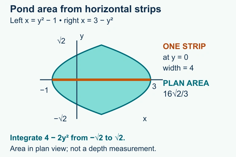Horizontal strips span the lens-shaped pond plan without changing formulas; their sum gives plan area rather than water depth. The coordinate diagram is a separate idealized plan; the landscape illustration supplies context.

Question 5: CRITICAL THINKING

3 pts

Consider the region R bounded by x = y² and x = 2 − y². (a) Find the y-value(s) where the curves intersect. (b) Set up and evaluate the dy-integral for the area of R. (c) Without computing the dx-integral explicitly, explain what difficulty arises if you attempt to find this area using dx-integration, and how many separate integrals would be required.

Show answer

Rubric (3 points): (a) [1 point] The curves intersect where

y^2

= 2 -

y^2

, so

2y^2

= 2,

y^2

= 1, and y = -1, 1. (b) [1 point] For -1 ≤ y ≤ 1, the right curve is x = 2 -

y^2

and the left curve is x =

y^2

, so A = ∫_{-1}^{1} [(2 -

y^2

) -

y^2

] dy = ∫_{-1}^{1} (2 -

2y^2

) dy = [2y - (2/3)

y^3

]_{-1}^{1} = (2 - 2/3) - (-2 + 2/3) = (4/3) - (-4/3) = 8/3. (c) [1 point] Using dx-integration requires inverting to y = ±√x (left curve) and y = ±√(2 - x) (right curve). The upper boundary switches from √x to √(2 - x) at x = 1 (where √x = √(2 - x)), so the integral from x = 0 to x = 2 must be split into two separate integrals: one from 0 to 1 (height 2√x) and one from 1 to 2 (height 2√(2 - x)).

SUMMARY

Lesson Summary

Summary

When a region in the xy-plane is bounded by curves more naturally expressed as functions of y, integrating with respect to y allows you to compute the enclosed area using a single integral of the form A = ∫ from c to d [f(y) − g(y)] dy, where f(y) is the right boundary and g(y) is the left boundary. The limits of integration are the y-coordinates of the intersection points, found by setting f(y) = g(y).

The key strategy is to sketch the region, identify which curve lies to the right at a test y-value, and confirm that the right-minus-left relationship holds throughout the interval. If the curves cross, split the integral at the crossing y-value. This technique avoids the multi-integral complications of dx-integration for sideways-opening curves, and it directly extends to the shell method for volumes of revolution and to iterated double integrals in multivariable calculus.