Finding the Area Between Curves Expressed as Functions of x - AP Calculus BC

SECTION 1

Historical Context & Motivation

The problem of finding areas enclosed by curves predates calculus itself, stretching back to ancient Greek mathematicians who exhausted polygonal approximations to pin down the areas of circles and parabolic segments. Archimedes employed the method of exhaustion—an ancestor of the modern limit process—to prove that the area of a parabolic segment equals four-thirds the area of the inscribed triangle. This feat demonstrated that areas bounded by curves could be computed rigorously, even without algebraic notation. The desire to generalize such calculations to arbitrary curves motivated centuries of mathematical development, culminating in the integral calculus of Newton and Leibniz.

~250 BCE • Archimedes' Quadrature of the Parabola

Archimedes computed the area of a parabolic segment using the method of exhaustion, the earliest rigorous technique for finding areas under curves.

1635 • Cavalieri's Principle of Indivisibles

Bonaventura Cavalieri proposed that areas could be decomposed into infinitely many parallel line segments, foreshadowing the Riemann sum approach to integration.

1666–1686 • Newton & Leibniz Formalize the Integral

Isaac Newton and Gottfried Wilhelm Leibniz independently developed the Fundamental Theorem of Calculus, linking antiderivatives to definite integrals and enabling systematic area computations.

1854 • Riemann's Formal Integral Definition

Bernhard Riemann formalized the definite integral as the limit of sums over partitions, providing the rigorous foundation underlying all area-between-curves calculations.

With the Fundamental Theorem of Calculus in hand, mathematicians could compute areas under single curves effortlessly. But the natural next question soon followed: how do we compute the area of the region trapped between two curves? This question arises constantly in physics (work done between force curves), economics (surplus between supply and demand), and engineering (cross-sectional areas). The elegant answer—integrating the vertical distance between the curves—is the subject of this lesson.

SECTION 2

Core Principles & Definitions

Before setting up any integral, you need a clear geometric picture and a handful of foundational ideas. The strategy for finding the area between two curves expressed as functions of x rests on the same Riemann sum intuition that underlies the definite integral: slice the region into thin vertical strips, approximate each strip's area, and sum across the interval. The following core principles formalize this approach and ensure you set up the integral correctly every time.

Top Minus Bottom

At each x-value in the interval, the height of a vertical strip is f(x) − g(x), where f(x) ≥ g(x). The area of the strip is [f(x) − g(x)] dx, and the total area is the integral of this expression over the interval.

Finding Intersection Points

The limits of integration are determined by solving f(x) = g(x). These intersection points mark where the two curves meet and enclose the region whose area you seek.

Splitting the Interval When Curves Swap

If f(x) ≥ g(x) on one sub-interval but g(x) ≥ f(x) on another, you must split the integral at each crossing point and always subtract the lower curve from the upper to keep each integrand non-negative.

Absolute Value Shortcut

Equivalently, the total area between two curves from x = a to x = b is ∫ₐᵇ |f(x) − g(x)| dx. This formulation automatically handles sign changes, though in practice you still identify crossing points to evaluate the integral.

✦

KEY TAKEAWAY

Think of the region between two curves as a stack of thin vertical rectangles. Each rectangle has a width of dx and a height equal to the gap between the upper and lower curves at that x-value. The definite integral acts like a precise assembly line, summing infinitely many of these infinitesimally thin rectangles into the exact area—much the way an engineer sums differential pressure readings across a surface to compute a total force.

SECTION 3

Visual Explanation

The diagram below illustrates the fundamental setup. Two continuous functions, f(x) (the upper curve in cyan) and g(x) (the lower curve in pink), are plotted on the same axes. The shaded region between them—from x = a to x = b—is the area we wish to compute. Notice the thin representative rectangle drawn at a sample x-value; its height is f(x) − g(x), and its width is dx.

The shaded region between f(x) (cyan) and g(x) (pink) from x = a to x = b. The yellow rectangle at a sample x-value shows the differential area element [f(x) − g(x)] dx that is summed by the definite integral.

The key geometric insight is that each vertical slice at position x contributes an area of [f(x) − g(x)] dx to the total enclosed area. As the width dx shrinks to zero and the number of slices grows to infinity, the Riemann sum converges to the definite integral ∫ₐᵇ [f(x) − g(x)] dx. This construction works regardless of whether the curves are above or below the x-axis—the only requirement is that you correctly identify which curve is on top at every x-value in the interval.

SECTION 4

Mathematical Framework

Let f and g be continuous functions on [a, b]. The formal derivation of the area formula begins with a Riemann sum. Partition [a, b] into n sub-intervals of equal width Δx = (b − a)/n, and choose sample points x₁*, x₂*, …, xₙ*. If f(xᵢ*) ≥ g(xᵢ*) for all i, the area of the i-th vertical strip is approximately [f(xᵢ*) − g(xᵢ*)] Δx. Summing over all strips and taking the limit as n → ∞ yields the definite integral.

AREA BETWEEN TWO CURVES (SINGLE INTERVAL)

A = ∫ₐᵇ [f(x) − g(x)] dx, where f(x) ≥ g(x) on [a, b]

f(x) is the upper curve, g(x) is the lower curve, and a and b are the x-coordinates of the intersection points (or specified bounds) that delimit the region.

AREA WITH CROSSING CURVES

A = ∫ₐᵇ |f(x) − g(x)| dx

When the curves cross one or more times inside [a, b], the absolute value ensures every strip contributes positive area. In practice, find all roots of f(x) = g(x) in (a, b), split the integral at those points, and integrate the appropriate difference on each sub-interval.

SPLIT-INTERVAL FORMULA

A = ∫ₐᶜ [f(x) − g(x)] dx + ∫ᶜᵇ [g(x) − f(x)] dx

Here c is the x-coordinate where the curves cross, i.e., f(c) = g(c). On [a, c], f is on top; on [c, b], g is on top. Each integral is set up so the integrand is non-negative.

⚠

Common Pitfall

Do not simply compute ∫ₐᵇ f(x) dx − ∫ₐᵇ g(x) dx if the curves cross inside (a, b). This yields the net signed area, which can be smaller than the geometric area because positive and negative contributions cancel. Always check for crossing points and split the integral accordingly.

SECTION 5

Handling Crossing Curves in Detail

The most frequent source of error on the AP exam is failing to account for regions where the curves swap positions. Consider two functions that intersect at three points: x = a, x = c, and x = b. The enclosed region consists of two sub-regions. On [a, c], suppose f lies above g, so the integrand is f(x) − g(x). On [c, b], g lies above f, so the integrand reverses to g(x) − f(x). The total area is the sum of these two integrals, and each integrand is guaranteed non-negative on its respective sub-interval.

Two curves crossing at x = c. Region I (cyan shading) has f on top; Region II (amber shading) has g on top. The total area is the sum of the two separate integrals, each with the correct top-minus-bottom orientation.

Step 1 — Find all intersections. Set f(x) = g(x) and solve for x. These solutions are your candidate limits and splitting points.
Step 2 — Determine which curve is on top. On each sub-interval between consecutive intersections, evaluate f and g at a test point to see which is larger.
Step 3 — Set up and evaluate separate integrals. Write each integral with (upper − lower) as the integrand, evaluate using the Fundamental Theorem, and add the results.

SECTION 6

Worked Example

Find the area of the region enclosed between f(x) = x + 2 and g(x) = x² on the interval where these curves form a closed region.

Area Between f(x) = x + 2 and g(x) = x²

1
Step 1 — Find the Intersection Points

Set f(x) = g(x): x + 2 = x². Rearranging gives x² − x − 2 = 0. Factoring: (x − 2)(x + 1) = 0, so x = −1 and x = 2. These are the limits of integration.

Intersection points: x = −1 and x = 2
2
Step 2 — Determine Which Curve Is on Top

Choose a test point between −1 and 2, say x = 0. Then f(0) = 0 + 2 = 2 and g(0) = 0² = 0. Since f(0) > g(0), the line f(x) = x + 2 lies above the parabola g(x) = x² on the entire interval [−1, 2].

Upper curve: f(x) = x + 2; Lower curve: g(x) = x²
3
Step 3 — Set Up the Integral

The area is A = ∫₋₁² [(x + 2) − x²] dx = ∫₋₁² (x + 2 − x²) dx.
4
Step 4 — Evaluate the Integral

Find the antiderivative: F(x) = x²/2 + 2x − x³/3. Now evaluate at the bounds: F(2) = 4/2 + 4 − 8/3 = 2 + 4 − 8/3 = 6 − 8/3 = 10/3. F(−1) = 1/2 − 2 − (−1/3) = 1/2 − 2 + 1/3 = −7/6. Therefore A = F(2) − F(−1) = 10/3 − (−7/6) = 10/3 + 7/6 = 20/6 + 7/6 = 27/6 = 9/2.

A = 9/2 = 4.5 square units

SECTION 7

Common Strategies, Strengths, and Pitfalls

Strategy / Situation	Strengths	Potential Pitfalls
Single integral when f ≥ g throughout [a, b]	Simplest setup; one antiderivative evaluation. Ideal when one curve is clearly above the other.	Fails if the curves cross inside the interval—net signed area ≠ geometric area.
Splitting the integral at crossing points	Always yields the correct geometric area. Essential when curves swap positions.	Requires solving f(x) = g(x) accurately; missing an intersection point will produce a wrong answer.
Using \|f(x) − g(x)\| directly	Conceptually clean; one formula covers all cases.	You still must find crossing points to remove the absolute value for antidifferentiation.
Integrating with respect to y instead of x	Sometimes reduces a multi-integral problem to a single integral (e.g., when boundaries are better described as functions of y).	Requires rewriting curves as x = h(y) and x = k(y). This lesson focuses on functions of x; the y-approach is covered separately.

Comparison of strategies for computing area between curves

🎯

EXAM TIP

On the AP Calculus BC exam, area-between-curves problems appear in both the multiple-choice and free-response sections. Free-response graders award separate points for correct limits of integration, a correct integrand with the proper top-minus-bottom orientation, and correct antidifferentiation. Even if you make an arithmetic slip in the final evaluation, you can still earn the majority of the rubric points by demonstrating a sound setup. Always sketch the region before writing the integral.

SECTION 8

Connections to Advanced Topics

Finding the area between curves in the xy-plane is the gateway to a family of more advanced integration applications that appear throughout AP Calculus BC and beyond. The same "slice, approximate, integrate" paradigm extends to computing volumes of solids of revolution (disk/washer and shell methods), volumes of solids with known cross-sections, arc lengths, and surface areas. In multivariable calculus, the idea generalizes to double integrals over planar regions, where you integrate a function f(x, y) over a domain D bounded by curves—a direct two-dimensional analogue of the single-variable area formula.

This Lesson	Advanced Extension
Area = ∫ₐᵇ [f(x) − g(x)] dx	Volume (washers) = π ∫ₐᵇ {[f(x)]² − [g(x)]²} dx, rotating the enclosed region about the x-axis
Vertical slices of width dx	Cross-sectional slices with known shape (squares, semicircles, equilateral triangles) perpendicular to an axis
f(x) ≥ g(x) determines the integrand sign	For polar curves r₁(θ) and r₂(θ), the area between them is ½ ∫ [r₁(θ)² − r₂(θ)²] dθ — an AP BC topic
Area is a scalar (always non-negative)	In economics, the signed integral ∫ [S(q) − D(q)] dq represents net surplus, where sign carries economic meaning

How area between curves connects to advanced calculus topics

Mastering the area-between-curves technique is essential not only for its own sake but because the conceptual framework—identifying bounds, choosing the right orientation (top − bottom vs. right − left), and splitting at crossing points—recurs in every subsequent integration application on the AP exam.

SECTION 9

Practice Problems

Question 1: CONCEPTUAL

Suppose you want to find the area between two continuous curves y = f(x) and y = g(x) from x = a to x = b. Which of the following correctly describes why you cannot simply compute ∫ₐᵇ f(x) dx − ∫ₐᵇ g(x) dx in all cases?

A. The Fundamental Theorem of Calculus does not apply when two functions are involved.
B. The difference ∫ₐᵇ f(x) dx − ∫ₐᵇ g(x) dx gives the net signed area, which can undercount the geometric area if the curves cross because positive and negative contributions cancel.
C. You must always use the absolute value |f(x) − g(x)| inside one integral, and splitting is never necessary.
D. The integral of a difference is not the same as the difference of the integrals.
E. The area between curves can only be computed using numerical methods, not antiderivatives.

Show answer (B)

The correct answer is B. When the curves cross inside [a, b], the function f(x) − g(x) changes sign. Integrating this signed quantity produces cancellation: the region where g > f contributes negative area that subtracts from the region where f > g, yielding a net signed area smaller than the total geometric area. Choice A is wrong because the FTC applies perfectly well to differences of functions. Choice C is partially correct in concept but wrong in claiming splitting is never necessary—you must split to remove the absolute value for antidifferentiation. Choice D is wrong because by the linearity of the integral, ∫[f − g] dx = ∫f dx − ∫g dx always holds. Choice E is wrong because antiderivatives are the standard evaluation method.

Question 2: BASIC CALCULATION

Find the area of the region enclosed between y = 4 − x² and y = x + 2.

A. 9/2
B. 7/2
C. 5
D. 11/2
E. 3

Show answer (A)

The correct answer is A. First, find the intersections: 4 − x² = x + 2 → x² + x − 2 = 0 → (x + 2)(x − 1) = 0, so x = −2 and x = 1. Test x = 0: 4 − 0 = 4 > 0 + 2 = 2, so 4 − x² is on top. The area is ∫₋₂¹ [(4 − x²) − (x + 2)] dx = ∫₋₂¹ (2 − x − x²) dx. The antiderivative is 2x − x²/2 − x³/3. At x = 1: 2 − 1/2 − 1/3 = 12/6 − 3/6 − 2/6 = 7/6. At x = −2: 2(−2) − (−2)²/2 − (−2)³/3 = −4 − 2 + 8/3 = −18/3 + 8/3 = −10/3. The area is 7/6 − (−10/3) = 7/6 + 20/6 = 27/6 = 9/2. Choice B (7/2) likely results from an arithmetic error in evaluating the antiderivative at the lower bound. Choice C (5) is incorrect and may result from dropping a fraction during evaluation. Choice D (11/2) could result from a sign error when subtracting the lower-bound evaluation. Choice E (3) is too small and likely results from using an incorrect integrand.

Question 3: INTERMEDIATE

Find the total area enclosed between f(x) = x³ − x and g(x) = 0 (the x-axis) on the interval [−1, 1].

A. 0
B. 1/4
C. 1/2
D. 1
E. 3/4

Show answer (C)

The correct answer is C. The function f(x) = x³ − x = x(x − 1)(x + 1) has roots at x = −1, 0, 1. On [−1, 0], test x = −0.5: (−0.5)³ − (−0.5) = −0.125 + 0.5 = 0.375 > 0, so f is above the x-axis. On [0, 1], test x = 0.5: 0.125 − 0.5 = −0.375 < 0, so f is below. Total area = ∫₋₁⁰ (x³ − x) dx + ∫₀¹ −(x³ − x) dx = ∫₋₁⁰ (x³ − x) dx + ∫₀¹ (x − x³) dx. Each integral evaluates to 1/4, so total area = 1/4 + 1/4 = 1/2. Choice A (0) is the net signed integral—it's zero by the odd symmetry of x³ − x, but it does not represent geometric area. Choice B (1/4) accounts for only one of the two sub-regions. Choice D (1) and E (3/4) result from evaluation errors.

Question 4: APPLIED

4 pts

A civil engineer models the cross-section of a river channel. The river surface is at height y = 6 and the riverbed follows y = x² − 1 for −√7 ≤ x ≤ √7 (all measurements in meters). Set up and evaluate a definite integral to find the cross-sectional area of the water in the channel. Show all work, including finding the limits of integration, setting up the integral, and evaluating it. Then interpret the result in context.

Show answer

Point 1 (Limits of Integration): Set x² − 1 = 6 → x² = 7 → x = ±√7. The water fills the cross-section from x = −√7 to x = √7. Point 2 (Integral Setup): The top curve is y = 6 (the water surface) and the bottom curve is y = x² − 1 (the riverbed). The cross-sectional area is A = ∫₋√₇^√7 [6 − (x² − 1)] dx = ∫₋√₇^√7 (7 − x²) dx. Point 3 (Antidifferentiation and Evaluation): By the even symmetry of the integrand, A = 2 ∫₀^√7 (7 − x²) dx = 2 [7x − x³/3] from 0 to √7 = 2 [7√7 − (√7)³/3] = 2 [7√7 − 7√7/3] = 2 · 7√7 · (1 − 1/3) = 2 · 7√7 · (2/3) = 28√7/3 ≈ 24.69 square meters. Point 4 (Interpretation): The cross-sectional area of approximately 24.69 m² represents the area of water visible in a vertical slice perpendicular to the river's flow. This value can be multiplied by the river's flow speed to estimate volumetric discharge rate (m³/s), a key quantity in hydrology and flood management. Parabolic bed y=x²−1 under waterline y=6, between x=±√7. The strip at x=1 has height 6; area is 28√7/3 m².

Parabolic bed y=x²−1 under waterline y=6, between x=±√7. The strip at x=1 has height 6; area is 28√7/3 m².

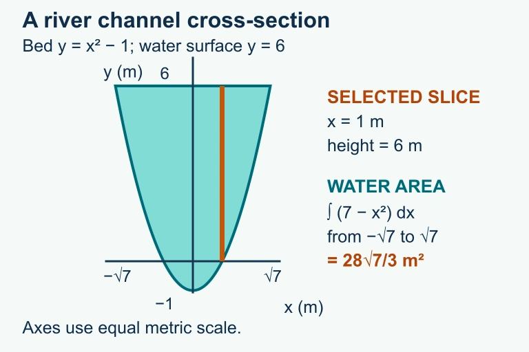The channel’s level water surface and parabolic bed enclose area 28√7/3 m² in the stated cross-section. The water face is an explanatory cutaway, not an unsupported real water wall.

Question 5: CRITICAL THINKING

3 pts

Let f(x) = sin(x) and g(x) = cos(x). Find the total area enclosed between these two curves on the interval [0, 2π]. Explain your strategy for handling the multiple crossings, identify all intersection points, and evaluate the resulting integrals.

Show answer

Point 1 (Intersection Points and Strategy): Set sin(x) = cos(x) → tan(x) = 1 → x = π/4 and x = 5π/4 on [0, 2π]. These two crossings divide [0, 2π] into three sub-intervals: [0, π/4], [π/4, 5π/4], and [5π/4, 2π]. On each sub-interval, determine which function is larger using test points. On [0, π/4], cos(x) > sin(x). On [π/4, 5π/4], sin(x) > cos(x). On [5π/4, 2π], cos(x) > sin(x). Point 2 (Integral Setup): A = ∫₀^{π/4} (cos x − sin x) dx + ∫_{π/4}^{5π/4} (sin x − cos x) dx + ∫_{5π/4}^{2π} (cos x − sin x) dx. Point 3 (Evaluation): First integral: [sin x + cos x] from 0 to π/4 = (√2/2 + √2/2) − (0 + 1) = √2 − 1. Second integral: [−cos x − sin x] from π/4 to 5π/4 = (√2/2 + √2/2) − (−√2/2 − √2/2) = √2 + √2 = 2√2. Third integral: [sin x + cos x] from 5π/4 to 2π = (0 + 1) − (−√2/2 − √2/2) = 1 + √2 = √2 + 1. Total area: (√2 − 1) + 2√2 + (√2 + 1) = 4√2 ≈ 5.657 square units.

SUMMARY

Lesson Summary

Summary

The area between two curves expressed as functions of x is computed by integrating the vertical distance between the upper curve f(x) and the lower curve g(x) across the interval [a, b]. The fundamental formula is A = ∫ₐᵇ [f(x) − g(x)] dx, valid when f(x) ≥ g(x) on the entire interval. The limits of integration are found by solving f(x) = g(x), which yields the intersection points that bound the enclosed region.

When the curves cross inside the interval, you must split the integral at each crossing point and ensure each sub-integral has the correct top-minus-bottom orientation. Failing to split produces the net signed area, not the geometric area. This technique—slicing a region into differential rectangles and summing—is the foundational pattern for computing volumes by washers and shells, volumes with known cross-sections, and area in polar coordinates—all key topics on the AP Calculus BC exam.