Exponential Models with
Differential Equations
Learn how the equation \(\dfrac{dy}{dt} = ky\) models growth and decay in nature, finance, and science.
What Is a Differential Equation?
A differential equation is an equation that relates a function to one or more of its derivatives. Instead of telling you the value of \(y\), it tells you how \(y\) changes.
Our goal: find the function \(y(t)\) that satisfies this relationship. This process is called solving the differential equation.
Why Exponential Models?
Many real-world quantities change at a rate proportional to their current size. This one simple idea produces the most important differential equation in calculus:
A cell culture where more cells create more growth events
 In the model y = 100e^(0.4t), the relative growth rate stays at 0.4 while total growth y′ = 0.4y increases with the population.
A cell culture where more cells create more growth events
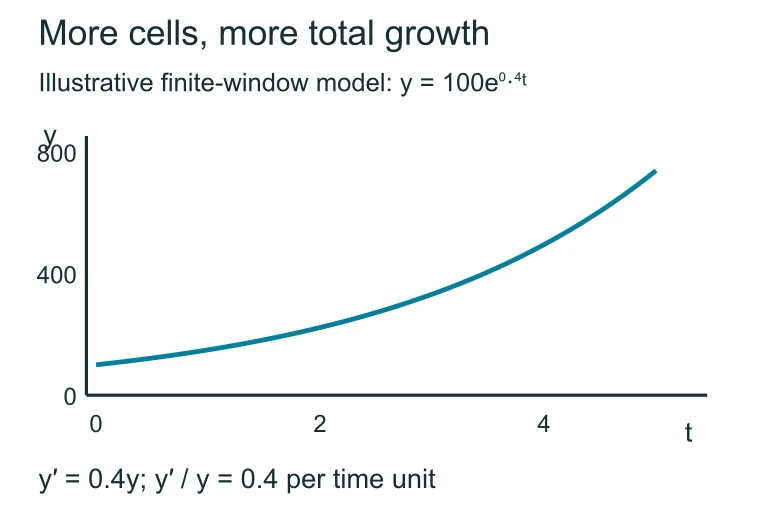 In the model y = 100e^(0.4t), the relative growth rate stays at 0.4 while total growth y′ = 0.4y increases with the population.
Relative rate versus total rate
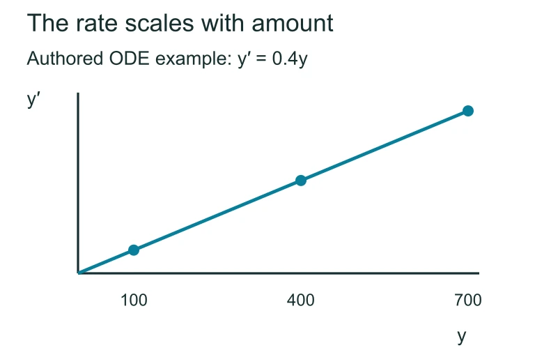 In the model y = 100e^(0.4t), the relative growth rate stays at 0.4 while total growth y′ = 0.4y increases with the population.
Visualizing Growth and Decay
Solving \(\dfrac{dy}{dt} = ky\) by Separation
Cooling coffee with temperature and rate shown separately
 With ambient temperature 22 °C and k > 0, T′ = −k(T − 22). A warmer liquid cools and a cooler liquid warms, both approaching ambient temperature.
Excess temperature decays toward zero
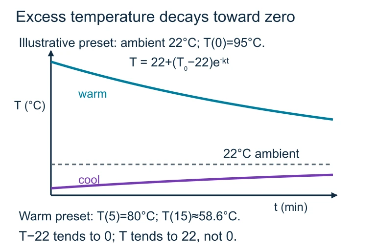 With ambient temperature 22 °C and k > 0, T′ = −k(T − 22). A warmer liquid cools and a cooler liquid warms, both approaching ambient temperature.
The General Solution
Continuous vs Discrete Growth
| Continuous | Discrete | |
|---|---|---|
| Model | \(y = y_0 e^{kt}\) | \(y = y_0 (1 + r)^t\) |
| Equation | \(\dfrac{dy}{dt} = ky\) | \(y_{n+1} = (1+r)\,y_n\) |
| Rate meaning | Instantaneous rate | Rate per period |
| AP Calculus focus | ★ Primary | Background |
How to Apply the Model
Example 1: Population Growth
A bacteria colony starts with 500 cells and grows at a rate proportional to its size. After 3 hours, there are 1500 cells. Find the population after 5 hours.
Example 1: Visualized
Example 2: Radioactive Decay
A substance has a half-life of 8 years. If the initial amount is 200 grams, how much remains after 20 years?
Example 3: Solving for Time
An investment of $2000 grows continuously at a rate of 6% per year. When will it reach $5000?
Doubling Time and Half-Life
$$t_d = \frac{\ln 2}{k}$$
$$t_h = \frac{\ln 2}{|k|}$$
Particular vs General Solutions
Common Mistakes to Avoid
Summary Reference Table
| Concept | Formula / Rule |
|---|---|
| Differential equation | \(\dfrac{dy}{dt} = ky\) |
| General solution | \(y = Ae^{kt}\) |
| Particular solution | \(y = y_0 e^{kt}\) |
| Doubling time | \(t_d = \dfrac{\ln 2}{k}\) |
| Half-life | \(t_h = \dfrac{\ln 2}{|k|}\) |
| Finding \(k\) | Use two data points and \(\ln\) |
| Finding time \(t\) | Isolate \(e^{kt}\), take \(\ln\) |
Question 1 of 5
If \(\dfrac{dy}{dt} = -0.3y\) and \(y(0) = 100\), what is \(y(t)\)?
Question 2 of 5
A population doubles every 5 years. What is the continuous growth rate \(k\)?
Question 3 of 5
A sample of 80 grams decays to 20 grams in 10 hours. What is the half-life?
Question 4 of 5
An investment grows continuously. It is worth $1000 at \(t = 0\) and $1500 at \(t = 4\). When will it be worth $3000?
Question 5 of 5
Which of the following differential equations does NOT have the solution \(y = Ce^{kt}\)?