Sketching Graphs of Functions and their Derivatives - AP Calculus AB

SECTION 1

Historical Context & Motivation

The relationship between a function and its rate of change has been a central concern of mathematics since the invention of calculus in the late seventeenth century. Before analytic formulas were commonplace, mathematicians relied on geometric reasoning — drawing tangent lines, measuring slopes, and inferring curvature — to understand how quantities evolve. The ability to move fluently between a function's graph and the graph of its derivative is not merely a classroom exercise; it is the conceptual backbone that connects algebraic differentiation rules to real-world interpretation of motion, optimization, and modeling.

1684 • Leibniz Publishes His Calculus

Gottfried Wilhelm Leibniz introduces the notation dy/dx and frames differentiation as finding the slope of a tangent, linking algebra to geometric curve-sketching.

1748 • Euler's Introductio

Leonhard Euler systematizes the study of functions and their graphs, laying the groundwork for the modern function concept and its graphical analysis.

1823 • Cauchy Formalizes Limits

Augustin-Louis Cauchy rigorously defines the derivative using limits, enabling precise statements about where functions increase, decrease, or change concavity.

1960s • Graphing in Calculus Education

University curricula formalize the 'first and second derivative tests' as standard tools for curve sketching, making derivative-graph correspondence a pillar of introductory calculus.

The central question this lesson addresses is both elegant and practical: given only the graph of a function, how can you deduce the graph of its derivative — and conversely, given the graph of a derivative, what can you infer about the original function's shape? Mastering this bidirectional reasoning is essential for the AP Calculus AB exam, where many free-response and multiple-choice questions present graphical information rather than explicit formulas.

SECTION 2

Core Principles & Definitions

The interplay between a function f and its derivative f′ rests on a small set of foundational ideas. Each principle converts a visual feature on one graph into a corresponding feature on the other, creating a precise translation dictionary between shape and sign.

Slope ↔ Value

The slope of f at any point x equals the y-value of f′ at that same x. A steep positive slope on f corresponds to a large positive value on f′.

Increasing / Decreasing

Where f is increasing, f′ > 0 (above the x-axis). Where f is decreasing, f′ < 0 (below the x-axis). The sign of f′ tells you the direction of f.

Extrema ↔ Zeros

Local maxima and minima of f occur where f′ = 0 or f′ is undefined, provided f′ changes sign. These are x-intercepts of the f′ graph.

Concavity ↔ Slope of f′

Where f is concave up, f′ is increasing; where f is concave down, f′ is decreasing. Inflection points of f correspond to extrema of f′.

Corners & Cusps

At a sharp corner or cusp on f, the derivative is undefined. On the f′ graph this appears as a jump discontinuity or vertical asymptote.

SECTION 3

Visual Explanation: From f to f′

The diagram below shows a function f (top) and its derivative f′ (bottom) aligned on the same x-axis. Study how features on the top graph translate to features on the bottom graph: where f has a local maximum, f′ crosses zero from positive to negative; where f has an inflection point, f′ has a local extremum.

The dashed vertical lines show how each critical feature of f (top) maps to a specific feature on f′ (bottom). A local maximum on f aligns with a zero-crossing (positive → negative) on f′, while an inflection point on f aligns with an extremum on f′.

Notice the shaded regions on the f′ graph. The green-tinted region where f′ > 0 corresponds to the interval on which f is climbing. The red-tinted region where f′ < 0 corresponds to the interval on which f is falling. This visual pairing is the single most important skill for the graphical reasoning questions on the AP exam.

A walking path crosses a ridge and hollow beside a staff-bearing observer. For f(x) = x³ − 3x, height, slope, and change in slope are different quantities. The extrema occur at x = −1 and 1; concavity changes at x = 0.

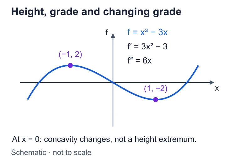For f(x) = x³ − 3x, height, slope, and change in slope are different quantities. The extrema occur at x = −1 and 1; concavity changes at x = 0.

SECTION 4

Mathematical Framework

The formal connections between f and f′ are encoded in the first derivative test and the second derivative test. These tests provide systematic criteria for classifying critical points and determining the overall shape of a graph without plotting hundreds of points.

FIRST DERIVATIVE TEST

If f′(c) = 0 and f′ changes from + to − at c, then f has a local maximum at c. If f′(c) = 0 and f′ changes from − to + at c, then f has a local minimum at c.

c is a critical number; the sign change of f′ determines whether f peaks or dips.

SECOND DERIVATIVE TEST

If f′(c) = 0 and f″(c) < 0, then f has a local maximum at c. If f′(c) = 0 and f″(c) > 0, then f has a local minimum at c.

f″(c) measures concavity at the critical point. Negative concavity (concave down) implies a peak; positive concavity (concave up) implies a valley.

CONCAVITY AND INFLECTION

f is concave up on (a, b) ⟺ f″(x) > 0 on (a, b) ⟺ f′ is increasing on (a, b). An inflection point occurs where f″ changes sign.

The equivalence among these three statements is the bridge connecting the f, f′, and f″ graphs.

When sketching f′ from f, estimate the slope of the tangent line at several representative x-values, plot those slope values, and connect them smoothly. When reconstructing f from f′, integrate qualitatively: note where f′ is positive (f rises), negative (f falls), zero (f has a horizontal tangent), increasing (f is concave up), and decreasing (f is concave down). These two procedures are inverses of one another and together form the complete graphical toolkit.

SECTION 5

Sign Charts & Feature Mapping

A sign chart is a compact summary tool that organizes the sign of f′ (and f″) across intervals, making it straightforward to determine the behavior of f. The table below codifies every possible combination of f′ and f″ signs and the resulting graph behavior.

f′ sign	f″ sign	f behavior	Graph shape
+ (positive)	+ (positive)	Increasing, concave up	Rising and bending upward ⌣
+ (positive)	− (negative)	Increasing, concave down	Rising and bending downward ⌢
− (negative)	+ (positive)	Decreasing, concave up	Falling and bending upward ⌣
− (negative)	− (negative)	Decreasing, concave down	Falling and bending downward ⌢

All four combinations of f′ and f″ signs determine the shape of the graph of f.

The four panels show the only possible shapes a smooth curve can take, determined by the combination of f′ and f″ signs. Transitions between these shapes occur at critical points and inflection points.

SECTION 6

Worked Example: Sketching f′ from f

Let f(x) = x³ − 3x. We will sketch the graph of f, derive f′ analytically, and verify the graphical correspondence.

Worked example

1
Step 1 — Find f′(x)

Differentiate: f′(x) = 3x² − 3 = 3(x² − 1) = 3(x − 1)(x + 1).

f′(x) = 3(x − 1)(x + 1)
2
Step 2 — Find critical points

Set f′(x) = 0: 3(x − 1)(x + 1) = 0 gives x = −1 and x = 1. Evaluate f at these: f(−1) = (−1)³ − 3(−1) = 2 and f(1) = 1 − 3 = −2.

Critical points: (−1, 2) and (1, −2)
3
Step 3 — First derivative sign chart

Test intervals: for x < −1, pick x = −2, f′(−2) = 3(4 − 1) = 9 > 0. For −1 < x < 1, pick x = 0, f′(0) = −3 < 0. For x > 1, pick x = 2, f′(2) = 3(4 − 1) = 9 > 0. So f increases on (−∞, −1), decreases on (−1, 1), and increases on (1, ∞).

Local max at x = −1, local min at x = 1
4
Step 4 — Concavity via f″

f″(x) = 6x. Set f″ = 0: x = 0. For x < 0, f″ < 0 (concave down); for x > 0, f″ > 0 (concave up). Thus x = 0 is an inflection point of f and corresponds to the minimum of f′.

Inflection point at (0, 0); f′ has minimum at x = 0
5
Step 5 — Sketch verification

The graph of f′(x) = 3x² − 3 is an upward-opening parabola with vertex at (0, −3) and x-intercepts at x = ±1. This matches our analysis: f′ > 0 outside [−1, 1], f′ < 0 inside (−1, 1), and f′ has its minimum at x = 0 — exactly the inflection point of f.

✓ The f′ parabola confirms all features of f.

SECTION 7

Common Pitfalls & Clarifications

Common Mistake	Why It's Wrong	Correct Reasoning
f′ = 0 always means an extremum	f′ must change sign to produce an extremum; f(x) = x³ has f′(0) = 0 but no max or min	Check sign change of f′ across the critical point
Confusing the y-value of f with the y-value of f′	A high point on f does not imply a high point on f′; the height of f′ reflects the slope, not the position	Read the f′ graph as slopes of f, not as positions of f
Assuming f′ has the same shape as f	Differentiation changes the degree and type of function; a cubic becomes a quadratic	Sketch f′ by estimating slopes at many points on f
Ignoring non-differentiable points	Corners, cusps, and vertical tangents on f create discontinuities on f′ that must be shown	Mark open circles or jumps on f′ at non-differentiable x-values

Frequent errors on AP exam graph-sketching questions

SECTION 8

Connections to Advanced Topics

The graph-sketching techniques in this lesson form the gateway to several deeper topics encountered in AP Calculus BC and beyond. Understanding how derivative graphs encode information about a function prepares you for the rigorous study of antiderivatives, accumulation functions, and differential equations.

AP Calculus AB Skill	Advanced Extension
Sketching f′ from f	Sketching f″ from f′ — extending the chain to higher-order derivatives (BC topic)
Reading f from f′ graph	Accumulation functions: F(x) = ∫₀ˣ f′(t) dt and the Fundamental Theorem of Calculus
Sign chart for f′ and f″	Phase-plane analysis in differential equations (university-level)
Identifying inflection points	Taylor polynomial error bounds depend on higher-derivative behavior (BC topic)

How AB curve-sketching skills extend into BC and university-level mathematics

In particular, the transition from "reading the derivative graph" to "computing definite integrals as signed areas under f′" is the conceptual leap that connects Unit 5 (Analytical Applications) to Unit 6 (Integration and Accumulation of Change) in the AP Calculus AB curriculum. If you can fluently move from f to f′ and back, the Fundamental Theorem of Calculus will feel like a natural formalization of what you already understand graphically.

SECTION 9

Practice Problems

Question 1: CONCEPTUAL

The graph of f′ is positive and decreasing on the interval (2, 5). Which of the following must be true about f on (2, 5)? (A) f is increasing and concave up (B) f is increasing and concave down (C) f is decreasing and concave up (D) f is decreasing and concave down (E) f is increasing and linear

A. f is increasing and concave up
B. f is increasing and concave down
C. f is decreasing and concave up
D. f is decreasing and concave down
E. f is increasing and linear

Show answer (B)

The correct answer is (B). Since f′ > 0, f is increasing. Since f′ is decreasing, f″ < 0, which means f is concave down. (A) is wrong because concave up requires f′ increasing, not decreasing. (C) and (D) are wrong because f′ > 0 means f is increasing, not decreasing. (E) is wrong because a linear function would have constant f′, not decreasing f′.

Question 2: BASIC CALCULATION

Let g(x) = x⁴ − 4x³. At how many points does the graph of g have an inflection point? (A) 0 (B) 1 (C) 2 (D) 3 (E) 4

A. 0
B. 1
C. 2
D. 3
E. 4

Show answer (C)

The correct answer is (C). Compute g″(x) = 12x² − 24x = 12x(x − 2). Setting g″ = 0 gives x = 0 and x = 2. Testing signs: for x < 0, g″ > 0; for 0 < x < 2, g″ < 0; for x > 2, g″ > 0. Since g″ changes sign at both x = 0 and x = 2, there are two inflection points. (A) is wrong because there are sign changes. (B) is wrong because both values produce sign changes, not just one. (D) and (E) are wrong because g″ is a quadratic with exactly two roots.

Question 3: INTERMEDIATE

The graph of f′ is a semicircle of radius 2 centered at (3, 0), above the x-axis for 1 < x < 5. The graph of f′ is zero for x ≤ 1 and x ≥ 5. Which of the following describes the graph of f? (A) f is constant on (−∞, 1), then decreasing on (1, 5), then constant on (5, ∞) (B) f is constant on (−∞, 1), then increasing on (1, 5), then constant on (5, ∞) (C) f is increasing on (−∞, 1), then constant on (1, 5), then increasing on (5, ∞) (D) f is increasing everywhere (E) f has a local maximum at x = 3

A. f is constant on (−∞, 1), then decreasing on (1, 5), then constant on (5, ∞)
B. f is constant on (−∞, 1), then increasing on (1, 5), then constant on (5, ∞)
C. f is increasing on (−∞, 1), then constant on (1, 5), then increasing on (5, ∞)
D. f is increasing everywhere
E. f has a local maximum at x = 3

Show answer (B)

The correct answer is (B). Where f′ = 0 (for x ≤ 1 and x ≥ 5), f has zero slope and is constant. Where f′ > 0 (on 1 < x < 5, since the semicircle is above the x-axis), f is increasing. The function rises by an amount equal to the area of the semicircle (½π(2²) = 2π) between x = 1 and x = 5. (A) is wrong because f′ > 0 means f increases, not decreases. (C) reverses the constant and increasing intervals. (D) is wrong because f′ = 0 outside (1, 5). (E) is wrong because f′ > 0 at x = 3, so f is increasing there, not at a maximum.

Question 4: APPLIED

A particle moves along the x-axis with velocity v(t) = t² − 6t + 8 for t ≥ 0. (a) Find all times t at which the particle changes direction. (b) On which intervals is the particle's speed increasing? (c) Sketch a qualitative graph of the position function x(t), assuming x(0) = 0, and label all critical points and inflection points.

Show answer

(a) [2 points] Set v(t) = 0: t² − 6t + 8 = (t − 2)(t − 4) = 0, so t = 2 and t = 4. Check sign changes: v > 0 on (0, 2), v < 0 on (2, 4), v > 0 on (4, ∞). The particle changes direction at t = 2 and t = 4. (b) [2 points] Speed = |v(t)|. Speed increases when v and a have the same sign. Compute a(t) = v′(t) = 2t − 6, so a = 0 at t = 3. On (0, 2): v > 0, a < 0 → speed decreasing. On (2, 3): v < 0, a < 0 → speed increasing. On (3, 4): v < 0, a > 0 → speed decreasing. On (4, ∞): v > 0, a > 0 → speed increasing. Speed is increasing on (2, 3) ∪ (4, ∞). (c) [2 points] x(t) has critical points at t = 2 (local max, since v changes + to −) and t = 4 (local min, since v changes − to +). The inflection point is at t = 3, where a(t) = v′(t) changes sign. The graph rises from (0, 0) to a local max at t = 2, falls to a local min at t = 4 with an inflection point at t = 3, then rises for t > 4. Concave down on (0, 3), concave up on (3, ∞).

Question 5: CRITICAL THINKING

Let f be a twice-differentiable function on (−∞, ∞) such that f′(x) > 0 for all x and f has exactly one inflection point. (a) Explain why f must be strictly increasing on its entire domain. (b) Describe the behavior of f′ and justify that f′ has exactly one local extremum. (c) Must f have a horizontal asymptote as x → ∞? Justify your answer with an example or counterexample.

Show answer

(a) [1 pt] Since f′(x) > 0 for all x, f is strictly increasing on (−∞, ∞) by the definition of the relationship between the sign of the first derivative and monotonicity. (b) [2 pts] An inflection point of f occurs where f″ changes sign, which is equivalent to f′ changing from increasing to decreasing (or vice versa). Since there is exactly one inflection point, f″ changes sign exactly once, meaning f′ has exactly one local extremum — either a local max (if f″ goes from + to −) or a local min (if f″ goes from − to +). (c) [1 pt] No, f need not have a horizontal asymptote. Counterexample: f(x) = x + arctan(x) satisfies f′(x) = 1 + 1/(1 + x²) > 0 for all x, and f″(x) = −2x/(1 + x²)² changes sign only at x = 0 (one inflection point). Yet f(x) → ∞ as x → ∞, so there is no horizontal asymptote. However, a function like f(x) = arctan(x) shows that a horizontal asymptote is possible. Therefore it is not required.