Using the Second Derivative Test to Determine Extrema - AP Calculus AB

SECTION 1

Historical Context & Motivation

The quest to find maximum and minimum values of functions stretches back centuries, long before the formal tools of calculus were codified. Ancient Greek geometers such as Euclid recognized extremal properties—for example, that among all rectangles with a given perimeter, the square encloses the greatest area—but lacked a general algorithmic procedure for locating extrema of arbitrary functions. The development of calculus in the late seventeenth century by Isaac Newton and Gottfried Wilhelm Leibniz finally gave mathematicians the language of derivatives with which to attack optimization problems systematically. The Second Derivative Test emerged as a natural refinement of first-derivative analysis, turning the geometric intuition about concavity into a precise criterion.

~300 BCE • Euclid's Extremal Geometry

Euclid demonstrated that certain geometric configurations maximize or minimize area and length, establishing early optimization reasoning without algebraic derivatives.

1684 • Leibniz Publishes the Calculus

Leibniz introduced the notation dy/dx and formal differentiation rules, enabling the systematic computation of tangent slopes and the identification of stationary points where dy/dx = 0.

1740s • Euler Formalizes Higher-Order Derivatives

Leonhard Euler expanded the framework of differential calculus to include second and higher-order derivatives, connecting the sign of d²y/dx² to the curvature of a graph and establishing the foundation for concavity analysis.

1797 • Lagrange's Théorie des Fonctions Analytiques

Joseph-Louis Lagrange presented a rigorous treatment of Taylor expansions and articulated the Second Derivative Test as a local criterion: if f′(c) = 0 and f″(c) > 0, then c is a local minimum—and vice versa for a maximum.

Modern Era • AP Calculus Curriculum

The Second Derivative Test is now a core topic in the AP Calculus AB framework, tested regularly in both multiple-choice and free-response contexts as an efficient method for classifying critical points.

The central question that the Second Derivative Test answers is deceptively simple: once you have found a point where the first derivative equals zero, how can you decide—without plotting the graph or constructing a sign chart—whether that point is a local maximum, a local minimum, or neither? The answer lies in the concavity of the function at that critical point, which is precisely what the second derivative measures.

SECTION 2

Core Principles & Definitions

Before applying the Second Derivative Test, you need a firm grasp of several foundational ideas that work together. A critical point of a function f occurs at x = c when f′(c) = 0 or f′(c) does not exist, provided f(c) is defined. The Second Derivative Test applies only at critical points where f′(c) = 0 and f″(c) exists; it leverages the sign of f″(c) to determine the nature of the extremum. Understanding the connection between the second derivative, concavity, and the shape of the graph is the conceptual engine behind the test.

Critical Points

Values x = c in the domain of f where f′(c) = 0 or f′(c) is undefined. These are the candidates for local extrema; the Second Derivative Test helps you classify those where f′(c) = 0.

Concavity

A function is concave up on an interval when f″(x) > 0 (the graph bends upward like a cup), and concave down when f″(x) < 0 (the graph bends downward like a cap). Concavity tells you how the slope itself is changing.

Second Derivative Test — Local Minimum

If f′(c) = 0 and f″(c) > 0, then f has a local minimum at x = c. The graph is concave up at c, so the stationary point sits at the bottom of a cup-shaped curve.

Second Derivative Test — Local Maximum

If f′(c) = 0 and f″(c) < 0, then f has a local maximum at x = c. The graph is concave down at c, so the stationary point sits at the top of a cap-shaped curve.

Inconclusive Case

If f′(c) = 0 and f″(c) = 0, the Second Derivative Test is inconclusive. You must revert to the First Derivative Test or another method to classify the critical point—it could be a maximum, minimum, or inflection point.

✦

KEY TAKEAWAY

Think of the Second Derivative Test like checking the shape of a bowl before placing a ball. If you find a flat spot (f′ = 0) on a surface that curves upward (f″ > 0), the ball settles into a local minimum—the bottom of the bowl. If the surface curves downward (f″ < 0), the ball rolls away from a local maximum—the top of a hill. If the surface is perfectly flat to second order (f″ = 0), you need more information to decide what happens.

SECTION 3

Visual Explanation

The curve f(x) (purple) has two critical points. At c₁, the graph is concave down (f″ < 0), producing a local maximum. At c₂, the graph is concave up (f″ > 0), producing a local minimum. Dashed horizontal tangent lines confirm f′ = 0 at each critical point.

Examine the diagram carefully. At every local maximum, the tangent line is horizontal and the curve lies below that tangent in a neighborhood of the point—this is the hallmark of concave-down behavior, corresponding to f″ < 0. Conversely, at every local minimum the tangent is horizontal and the curve lies above the tangent nearby, reflecting concave-up behavior where f″ > 0. The Second Derivative Test distills this visual observation into a single algebraic check: evaluate f″ at the critical point and read off the sign. When f″(c) = 0, the curve may be transitioning between concavity types (an inflection point with zero slope), or it may still be an extremum—the test simply cannot tell, and you must investigate further.

SECTION 4

Mathematical Framework

The rigorous justification of the Second Derivative Test rests on the local quadratic approximation provided by Taylor's theorem. If f is twice differentiable near x = c and f′(c) = 0, the Taylor expansion about c gives f(x) ≈ f(c) + ½ f″(c)(x − c)². When f″(c) > 0, this approximation is an upward-opening parabola centered at c, guaranteeing that f(x) > f(c) for x near (but not equal to) c—hence a local minimum. The analogous argument with f″(c) < 0 yields a downward-opening parabola and a local maximum. Below are the formal statements you must internalize for the AP exam.

CRITICAL POINT CONDITION

f′(c) = 0

A necessary condition for the Second Derivative Test to apply. The point x = c must be in the domain of f, and f′(c) must equal zero (not merely undefined).

LOCAL MINIMUM CRITERION

f′(c) = 0 and f″(c) > 0 ⟹ f has a local minimum at x = c

Positive second derivative means the graph is concave up at c. Combined with a horizontal tangent, this forces a valley (local minimum).

LOCAL MAXIMUM CRITERION

f′(c) = 0 and f″(c) < 0 ⟹ f has a local maximum at x = c

Negative second derivative means the graph is concave down at c. Combined with a horizontal tangent, this forces a peak (local maximum).

INCONCLUSIVE CASE

f′(c) = 0 and f″(c) = 0 ⟹ test is inconclusive

When the second derivative vanishes at a critical point, the local quadratic approximation is degenerate. Use the First Derivative Test (sign-chart method) or higher-order derivative analysis to classify the point.

💡

AP Exam Tip

On the AP Calculus AB exam, free-response rubrics typically award separate points for (1) finding the critical point, (2) computing f″(c), (3) stating the sign of f″(c), and (4) concluding with a properly justified classification. Always write a concluding sentence such as: "Because f′(c) = 0 and f″(c) > 0, f has a local minimum at x = c." Omitting the justification can cost you a point even if your numerical work is correct.

SECTION 5

Classifying Critical Points — Decision Flowchart

When you encounter an optimization or curve-sketching problem on the AP exam, you need a systematic procedure for classifying every critical point. The flowchart below encodes the full decision logic: first locate the critical points, then attempt the Second Derivative Test, and fall back to the First Derivative Test when the second derivative is zero or does not exist.

Start at the top by finding critical points where f′(c) = 0. Compute f″(c) and branch according to its sign. If the Second Derivative Test is inconclusive (f″(c) = 0), fall back to the First Derivative Test by analyzing the sign change of f′ around c.

Condition	f″(c) > 0	f″(c) < 0	f″(c) = 0
Concavity at c	Concave up	Concave down	Indeterminate
Conclusion	Local minimum	Local maximum	Test fails — use FDT
Graph shape	Valley (∪)	Peak (∩)	Could be ∪, ∩, or flat

Summary of Second Derivative Test outcomes

SECTION 6

Worked Example

Let us apply the Second Derivative Test to a polynomial function that arises frequently in AP problems. Consider f(x) = 2x³ − 9x² + 12x − 4. We will find all critical points and classify each as a local maximum, local minimum, or neither.

Classify the extrema of f(x) = 2x³ − 9x² + 12x − 4

1
Step 1 — Compute the first derivative

Differentiate f(x) term by term using the power rule: f′(x) = 6x² − 18x + 12. Factor out the common factor of 6: f′(x) = 6(x² − 3x + 2) = 6(x − 1)(x − 2).

f′(x) = 6(x − 1)(x − 2)
2
Step 2 — Find the critical points

Set f′(x) = 0 and solve: 6(x − 1)(x − 2) = 0 gives x = 1 and x = 2. Since f′ is a polynomial (exists everywhere), these are the only critical points.

Critical points: x = 1 and x = 2
3
Step 3 — Compute the second derivative

Differentiate f′(x) = 6x² − 18x + 12 to obtain f″(x) = 12x − 18.

f″(x) = 12x − 18
4
Step 4 — Evaluate f″ at each critical point

At x = 1: f″(1) = 12(1) − 18 = −6. Since f″(1) < 0, the graph is concave down at x = 1. At x = 2: f″(2) = 12(2) − 18 = 6. Since f″(2) > 0, the graph is concave up at x = 2.

f″(1) = −6 < 0 ; f″(2) = 6 > 0
5
Step 5 — State the conclusions with justification

By the Second Derivative Test: because f′(1) = 0 and f″(1) = −6 < 0, f has a local maximum at x = 1 with value f(1) = 2(1)³ − 9(1)² + 12(1) − 4 = 1. Because f′(2) = 0 and f″(2) = 6 > 0, f has a local minimum at x = 2 with value f(2) = 2(8) − 9(4) + 12(2) − 4 = 0.

Local max at (1, 1); Local min at (2, 0)

💡

Exam Writing Tip

Notice how each conclusion sentence includes three elements: the condition f′(c) = 0, the sign of f″(c), and the classification. This mirrors the rubric structure that AP graders use. Practice writing conclusions in this format until it becomes automatic.

SECTION 7

Second Derivative Test vs. First Derivative Test

Both the First Derivative Test and the Second Derivative Test serve the same ultimate purpose—classifying critical points as local maxima, local minima, or neither—but they differ in their approach, computational requirements, and domain of applicability. Understanding when each test is preferable is important for efficiency on the AP exam and for handling cases where one test fails.

Feature	First Derivative Test	Second Derivative Test
What you analyze	Sign of f′ on intervals around c	Value of f″ at c alone
Requires	f′ exists near c (not necessarily at c)	f″(c) exists and f′(c) = 0
Works when f′(c) DNE?	Yes — e.g., cusps, corners	No — requires f′(c) = 0
Fails when?	Never (always gives a classification if sign chart is done correctly)	When f″(c) = 0 (inconclusive)
Computational cost	Must test multiple points in intervals	Single evaluation of f″(c)
Best suited for	Functions with non-differentiable critical points; when f″ is hard to compute	Smooth functions where f″ is easy to compute; many critical points

Comparison of the two primary tests for classifying extrema

⚡

STRATEGIC INSIGHT

Think of the Second Derivative Test as a quick diagnostic and the First Derivative Test as a comprehensive scan. In engineering, you run the quick test first (compute one number), and if it comes back inconclusive, you order the full workup (build the sign chart). On the AP exam, start with the Second Derivative Test for speed; fall back to the First Derivative Test only when f″(c) = 0 or when the problem specifically asks for a first-derivative analysis.

SECTION 8

Connections to Advanced Theory

The Second Derivative Test you learn in AP Calculus AB is actually a special case of far more powerful classification tools that appear in multivariable calculus, optimization theory, and differential geometry. Recognizing these connections will deepen your understanding and prepare you for the mathematical landscape beyond the AP course.

AP Calculus AB Concept	Advanced Generalization
f″(c) > 0 ⟹ local min	In multivariable calculus, the Hessian matrix H(c) replaces f″(c). If ∇f(c) = 0 and H(c) is positive definite, then c is a local minimum.
f″(c) < 0 ⟹ local max	If ∇f(c) = 0 and H(c) is negative definite, then c is a local maximum.
f″(c) = 0 ⟹ inconclusive	When the Hessian is indefinite, the critical point is a saddle point. When the Hessian is singular (det = 0), the test is again inconclusive and higher-order analysis is needed.
Optimization on open intervals	Constrained optimization uses Lagrange multipliers with a bordered Hessian to classify extrema on surfaces and curves in higher dimensions.

From single-variable to multivariable: how the Second Derivative Test generalizes

Another important connection is to Taylor polynomial approximations that appear in BC Calculus and beyond. The Second Derivative Test is essentially reading off the curvature of the best-fit parabola at a critical point. When f″(c) = 0, the parabolic approximation degenerates, and you need the cubic or higher-order terms of the Taylor expansion to determine the behavior—this is exactly why the test becomes inconclusive. Appreciating this connection between local polynomial approximation and extremum classification turns the Second Derivative Test from a memorized rule into a deeply understood principle.

SECTION 9

Practice Problems

Question 1: CONCEPTUAL

Suppose f is twice differentiable at x = 3, f′(3) = 0, and f″(3) = −7. Which of the following must be true?

A. f has a local minimum at x = 3.
B. f has a local maximum at x = 3.
C. f has an inflection point at x = 3.
D. f is concave up at x = 3.
E. The Second Derivative Test is inconclusive at x = 3.

Show answer (B)

Answer: B. By the Second Derivative Test, since f′(3) = 0 and f″(3) = −7 < 0, the function is concave down at x = 3, so f has a local maximum there. Choice A is wrong because f″(3) < 0 indicates concave down, not concave up (which would be needed for a local minimum). Choice C is wrong because an inflection point requires a change in concavity, not merely a critical point. Choice D contradicts f″(3) < 0, which means concave down. Choice E is wrong because the test is inconclusive only when f″(c) = 0, and here f″(3) = −7 ≠ 0.

Question 2: BASIC CALCULATION

Let g(x) = x⁴ − 8x² + 16. Find all critical points of g and use the Second Derivative Test to classify them. At which x-value does g have a local minimum?

A. x = 0 only
B. x = −2 and x = 2 only
C. x = 0, x = −2, and x = 2
D. x = −2 only
E. x = 2 only

Show answer (B)

Answer: B. Compute g′(x) = 4x³ − 16x = 4x(x² − 4) = 4x(x − 2)(x + 2), giving critical points x = 0, x = 2, and x = −2. Then g″(x) = 12x² − 16. Evaluating: g″(0) = −16 < 0 (local maximum at x = 0), g″(2) = 12(4) − 16 = 32 > 0 (local minimum at x = 2), g″(−2) = 12(4) − 16 = 32 > 0 (local minimum at x = −2). So g has local minima at x = −2 and x = 2. Choice A is wrong because x = 0 is a local maximum, not a minimum. Choice C is wrong because x = 0 is not a local minimum. Choices D and E each identify only one of the two local minima and miss the other.

Question 3: INTERMEDIATE

Consider h(x) = x³ − 3x² + 3x − 1. Find the critical point(s) and apply the Second Derivative Test. What can you conclude?

A. h has a local minimum at x = 1.
B. h has a local maximum at x = 1.
C. The Second Derivative Test is inconclusive at x = 1; the First Derivative Test shows no extremum.
D. h has no critical points.
E. The Second Derivative Test is inconclusive at x = 1; the First Derivative Test shows a local minimum.

Show answer (C)

Answer: C. First, note that h(x) = (x − 1)³. Differentiating: h′(x) = 3(x − 1)² and h″(x) = 6(x − 1). Setting h′(x) = 0 gives x = 1 as the only critical point. Evaluating h″(1) = 6(0) = 0, so the Second Derivative Test is inconclusive. Applying the First Derivative Test: h′(x) = 3(x − 1)² ≥ 0 for all x, meaning h′ does not change sign at x = 1. Therefore x = 1 is neither a local maximum nor a local minimum—it is an inflection point. Choice A is wrong because h has no local minimum. Choice B is wrong for the same reason. Choice D is wrong because x = 1 is indeed a critical point (h′(1) = 0). Choice E is wrong because the First Derivative Test reveals no sign change, hence no local minimum.

Question 4: APPLIED

5 pts

A manufacturer designs an open-top box by cutting equal squares of side length x inches from each corner of a 12-inch by 18-inch sheet of metal and folding up the sides. (a) Show that the volume of the box is V(x) = x(12 − 2x)(18 − 2x). (b) Find all critical points of V on the interval (0, 6). (c) Use the Second Derivative Test to classify each critical point. (d) State the dimensions that maximize the volume and give the maximum volume.

Show answer

Rubric (5 points): Point 1 (Part a): After cutting squares of side x from each corner, the base has dimensions (12 − 2x) by (18 − 2x), and the height is x. Therefore V(x) = x(12 − 2x)(18 − 2x). Expanding: V(x) = x(216 − 24x − 36x + 4x²) = 4x³ − 60x² + 216x. Point 2 (Part b): V′(x) = 12x² − 120x + 216 = 12(x² − 10x + 18). Using the quadratic formula: x = (10 ± √(100 − 72))/2 = (10 ± √28)/2 = 5 ± √7. So x = 5 − √7 ≈ 2.354 and x = 5 + √7 ≈ 7.646. Only x = 5 − √7 lies in (0, 6). Point 3 (Part c — computing f″): V″(x) = 24x − 120. At x = 5 − √7: V″(5 − √7) = 24(5 − √7) − 120 = 120 − 24√7 − 120 = −24√7 ≈ −63.5. Point 4 (Part c — conclusion): Since V′(5 − √7) = 0 and V″(5 − √7) = −24√7 < 0, by the Second Derivative Test, V has a local maximum at x = 5 − √7. Because this is the only critical point on (0, 6) and V(0) = V(6) = 0, this local maximum is also the absolute maximum on [0, 6]. Point 5 (Part d): With x = 5 − √7, the dimensions are: height = 5 − √7 ≈ 2.354 in, width = 12 − 2(5 − √7) = 2 + 2√7 ≈ 7.292 in, length = 18 − 2(5 − √7) = 8 + 2√7 ≈ 13.292 in. Maximum volume: V(5 − √7) = (5 − √7)(2 + 2√7)(8 + 2√7). Computing numerically: V ≈ 2.354 × 7.292 × 13.292 ≈ 228.2 in³. An 18 in by 12 in sheet with four equal square corner cuts and a schematic folded open box. Height is x and base sides are 18−2x and 12−2x.

An 18 in by 12 in sheet with four equal square corner cuts and a schematic folded open box. Height is x and base sides are 18−2x and 12−2x.

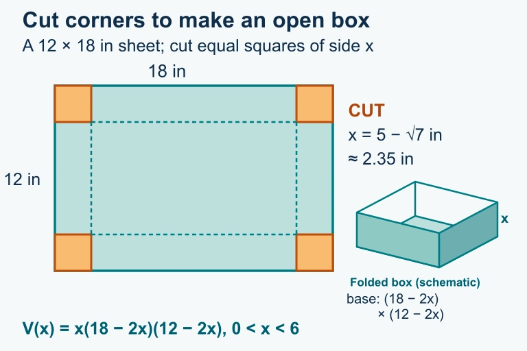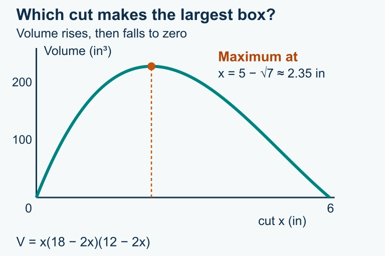An 18 in by 12 in sheet produces an open box of volume V=x(18−2x)(12−2x), maximized at x=5−√7 in. Volume in cubic inches versus cut length in inches for an 18 in by 12 in sheet. The maximum occurs at x=5−√7, about 2.354 in.

Volume in cubic inches versus cut length in inches for an 18 in by 12 in sheet. The maximum occurs at x=5−√7, about 2.354 in.

An 18 in by 12 in sheet produces an open box of volume V=x(18−2x)(12−2x), maximized at x=5−√7 in.

Question 5: CRITICAL THINKING

3 pts

Let f(x) = x⁴ and g(x) = −x⁴. Both functions have f′(0) = 0 and f″(0) = 0 (and similarly for g). Yet f has a local minimum at x = 0 and g has a local maximum at x = 0. Explain why the Second Derivative Test fails for these functions, and describe a general strategy for classifying critical points when f″(c) = 0. Your answer should reference the behavior of the first derivative.

Show answer

Rubric (3 points): Point 1 — Explain why SDT fails: The Second Derivative Test relies on the sign of f″(c) to determine concavity at the critical point. When f″(c) = 0, the local quadratic approximation f(c) + ½f″(c)(x − c)² degenerates to a constant, providing no curvature information. Both f(x) = x⁴ and g(x) = −x⁴ satisfy f″(0) = 0, yet they have opposite extremal behavior, demonstrating that f″(c) = 0 carries no information about the type of extremum. Point 2 — First Derivative Test strategy: When the Second Derivative Test is inconclusive, apply the First Derivative Test by examining the sign of f′(x) on either side of c. For f(x) = x⁴, f′(x) = 4x³ changes from negative to positive at x = 0, confirming a local minimum. For g(x) = −x⁴, g′(x) = −4x³ changes from positive to negative, confirming a local maximum. Point 3 — General principle: The First Derivative Test is universally applicable and never inconclusive: if f′ changes from positive to negative at c, there is a local maximum; if f′ changes from negative to positive, there is a local minimum; if there is no sign change, c is neither. Alternatively, one can examine higher-order derivatives: the first nonzero derivative f⁽ⁿ⁾(c) determines the behavior—if n is even and f⁽ⁿ⁾(c) > 0, it is a local minimum; if n is even and f⁽ⁿ⁾(c) < 0, it is a local maximum; if n is odd, c is an inflection point.

SUMMARY

Lesson Summary

Summary

The Second Derivative Test provides an efficient method for classifying critical points where f′(c) = 0. If f″(c) > 0, the function is concave up and the critical point is a local minimum. If f″(c) < 0, the function is concave down and the critical point is a local maximum. When f″(c) = 0, the test is inconclusive and you must fall back to the First Derivative Test.

On the AP exam, remember the three-part justification: state that f′(c) = 0, give the sign of f″(c), and write the classification. The Second Derivative Test is fastest when f″ is easy to compute, but always keep the First Derivative Test in your toolkit for cases where the second derivative vanishes or does not exist. Mastering both tests—and knowing when to deploy each—is essential for full credit on free-response optimization problems.