Modeling Situations with Differential Equations - AP Calculus AB

SECTION 1

Historical Context & Motivation

Long before calculus had a formal language, scientists and philosophers grappled with a deceptively simple question: if you know how fast something changes, can you predict what it will become? A differential equation is precisely a mathematical statement that relates a function to its own rate of change, and the art of constructing such equations from physical or biological scenarios is called modeling. The historical arc of this idea spans centuries, connecting Newton's laws of motion, population biology, radioactive decay, and financial mathematics under a single conceptual umbrella.

1687 • Newton's Principia

Isaac Newton published the Principia Mathematica, expressing the second law of motion as F = ma—essentially a differential equation relating force to the second derivative of position.

1798 • Malthus on Population

Thomas Malthus proposed that populations grow in proportion to their current size, leading to the exponential growth model dP/dt = kP, one of the simplest and most iconic differential equations.

1838 • Verhulst's Logistic Model

Pierre-François Verhulst refined Malthus's model by introducing a carrying capacity, yielding the logistic equation dP/dt = kP(1 − P/L), which accounts for limited resources.

1896 • Radioactive Decay Quantified

Henri Becquerel's discovery of radioactivity eventually led to the decay model dN/dt = −λN, establishing differential equations as the language of nuclear physics.

Modern Era • Computational Modeling

Today, differential equations underpin climate models, epidemiological forecasts (SIR models), financial option pricing (Black-Scholes), and countless engineering systems—all built from the same core principle of relating quantities to their rates.

The central challenge that unites all these examples is: given a verbal or physical description of how a quantity changes over time, how do we translate that description into a precise differential equation? This is exactly the skill tested on the AP Calculus AB exam, and it is the focus of this lesson.

SECTION 2

Core Principles & Definitions

Before you can model a situation with a differential equation, you need a firm grasp of what these equations are and how they encode information about change. At its core, a differential equation is an equation that contains a derivative of an unknown function. Your job in modeling is to interpret a real-world scenario and express the relationship between a quantity and its rate of change as such an equation.

Differential Equation

An equation involving an unknown function y and one or more of its derivatives (dy/dt, d²y/dt², …). On the AP exam, you'll work exclusively with first-order ordinary differential equations (ODEs).

Rate of Change as a Derivative

Phrases like "the rate of change of y is proportional to y" translate directly to dy/dt = ky. The derivative dy/dt captures the instantaneous rate at which y changes with respect to time t.

Proportionality Constant

The constant k in dy/dt = ky determines growth (k > 0) or decay (k < 0). Its units ensure dimensional consistency—for example, if y is in grams and t in years, k has units year⁻¹.

Initial Condition

A differential equation alone typically has infinitely many solutions. An initial condition such as y(0) = y₀ pins down a unique particular solution from the family of general solutions.

Solution of a DE

A solution is a function y(t) that, when substituted into the differential equation, produces a true statement for all t in the domain. Verifying a solution means differentiating and checking.

✦

KEY TAKEAWAY

Think of a differential equation as a recipe that describes how a quantity changes rather than what it equals. Just as a GPS gives you turn-by-turn directions (rates of change) rather than your final address (explicit function), a differential equation tells you the velocity of change at every instant. Solving the equation is like following the directions to find the destination—the explicit function y(t).

SECTION 3

Visual Explanation: From Words to Equations

The diagram below illustrates the modeling pipeline: you start with a verbal description of a real-world phenomenon, identify the key quantities and their relationships, and produce a differential equation. Arrows indicate the logical flow, and color coding distinguishes the verbal, mathematical, and solution stages.

The modeling pipeline flows from left to right: identify variables (Step 1, blue), write the differential equation (Step 2, violet), then solve or analyze (Step 3, green). The bottom row shows the three most common verbal-to-mathematical translations you will encounter on the AP exam.

Notice that the modeling process is fundamentally one of translation. You are converting English phrases—"the rate of change is proportional to," "decreases at a rate equal to"—into precise mathematical notation. Every AP free-response question on this topic will test your ability to perform this translation accurately, so learning to recognize the common verbal cues shown in the lower portion of the diagram is essential. The phrase "rate of change" always maps to a derivative, and "proportional to" always introduces a constant of proportionality multiplied by some expression.

SECTION 4

Mathematical Framework

In AP Calculus AB, you will model situations using first-order differential equations of the form dy/dt = f(t, y). The mathematical structure of the right-hand side f(t, y) determines the type of model and, ultimately, the behavior of the solution. Below are the fundamental forms you must master, each arising from a distinct class of real-world scenarios.

EXPONENTIAL GROWTH / DECAY

dy/dt = ky

Here y is the quantity (population, mass, amount), t is the independent variable (usually time), and k is the constant of proportionality. If k > 0 the quantity grows; if k < 0 it decays. The general solution is y(t) = y₀e^kt.

NEWTON'S LAW OF COOLING

dT/dt = k(T − Tₛ)

T is the temperature of the object, Tₛ is the surrounding (ambient) temperature, and k is a negative constant. The rate of temperature change is proportional to the difference between the object's temperature and its environment.

LOGISTIC GROWTH

dy/dt = ky(1 − y/L)

L is the carrying capacity (maximum sustainable population), and the factor (1 − y/L) acts as a braking mechanism. When y is small relative to L, the model approximates exponential growth; as y approaches L, the growth rate approaches zero.

GENERAL FIRST-ORDER MODEL

dy/dt = f(t, y), y(t₀) = y₀

This is the most general form you'll see on the AP exam. The function f(t, y) can be any expression in t and y, and the initial condition y(t₀) = y₀ selects the unique solution curve from the family of all solutions.

💡

AP Exam Tip

On the AP exam, you are rarely asked to solve a differential equation beyond the separable case. More often, you must set up the correct equation from a verbal description, verify that a given function is a solution, or use a slope field or Euler's method to approximate the solution. Modeling—translating words into dy/dt = f(t, y)—is the critical first step.

SECTION 5

Detailed Breakdown of Model Types

Different verbal descriptions lead to distinct mathematical structures. The diagram below compares the solution curves of the three primary models side by side on the same axes, making their qualitative differences immediately visible. Understanding these shapes—exponential, logistic, and cooling/heating—will help you quickly identify which model a problem is asking for.

Three fundamental model types plotted on the same axes. The exponential growth curve (pink) accelerates without bound. The logistic curve (cyan) follows the same trajectory initially but bends toward the carrying capacity L. The cooling curve (gold) begins above ambient temperature and decays toward Tₛ.

Model	Verbal Cue	Differential Equation	Solution Behavior
Exponential Growth	"rate proportional to current amount"	dy/dt = ky, k > 0	Unbounded increase; y → ∞
Exponential Decay	"rate proportional to current amount" (decreasing)	dy/dt = ky, k < 0	Decays toward zero; y → 0
Logistic Growth	"rate proportional to product of y and (L − y)"	dy/dt = ky(1 − y/L)	S-shaped; y → L as t → ∞
Newton's Cooling	"rate proportional to difference from surroundings"	dT/dt = k(T − Tₛ)	T approaches Tₛ exponentially
Constant Rate	"changes at a constant rate of 5 per minute"	dy/dt = C	Linear growth or decline

Summary of the five most common differential equation models on the AP Calculus AB exam.

A stirred transparent tank has one upper inlet and one lower outlet with a valve. The exact diagram links its 100 L salt balance to a computed approach to equilibrium. A well-mixed 100 L tank receives and releases 4 L/min. Salt enters at 2 kg/min and leaves at 0.04S kg/min, giving S′ = 2 − 0.04S.

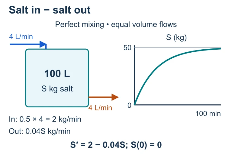A well-mixed 100 L tank receives and releases 4 L/min. Salt enters at 2 kg/min and leaves at 0.04S kg/min, giving S′ = 2 − 0.04S.

SECTION 6

Worked Example: Modeling a Population

A biologist observes that a population of bacteria in a culture dish grows at a rate proportional to both the current population and the fraction of the carrying capacity that remains unused. The carrying capacity of the dish is 10,000 bacteria. At time t = 0, the population is 500 bacteria. Write a differential equation that models this situation, identify the type of model, and determine the population at the instant when the growth rate is maximized.

Modeling a Bacterial Population

1
Step 1 — Identify Variables and Given Information

Let P(t) represent the population at time t. The carrying capacity is L = 10,000. The initial condition is P(0) = 500. The problem states that the growth rate is proportional to the current population and the fraction of unused capacity, which is (1 − P/L).
2
Step 2 — Translate the Verbal Description into a DE

"Rate of change" translates to dP/dt. "Proportional to the current population and the fraction of unused capacity" means dP/dt equals a constant k multiplied by P and by (1 − P/L). This gives us the logistic differential equation:

dP/dt = kP(1 − P/10000)
3
Step 3 — Identify the Model Type

This is the logistic growth model. The right-hand side is a quadratic function of P (it can be expanded to kP − kP²/10000), and the solution curve will be S-shaped, approaching L = 10,000 as t → ∞.
4
Step 4 — Find the Population When Growth Rate is Maximum

The growth rate dP/dt = kP(1 − P/10000) is a downward-opening parabola in P with roots at P = 0 and P = 10,000. A quadratic aP − bP² is maximized at its vertex, which occurs at P = a/(2b). Here a = k and b = k/10000, so P = k / (2 × k/10000) = 10000/2 = 5000. Alternatively, recall the general result: for the logistic model, the maximum growth rate occurs at P = L/2.

The growth rate is maximized when P = 5,000 bacteria.
5
Step 5 — Verify and Interpret

When P = 5,000, the factor P/L = 1/2 and (1 − P/L) = 1/2, so dP/dt = k × 5000 × 0.5 = 2500k. For any other value of P, the product P(1 − P/L) is smaller. This makes intuitive sense: the population is large enough to reproduce quickly but far enough from the resource limit that competition hasn't yet slowed growth significantly.

SECTION 7

Strengths and Limitations of DE Models

Differential equation models are powerful precisely because they reduce complex real-world phenomena to simple mathematical relationships. However, every model is an approximation, and recognizing the assumptions behind each equation is just as important as being able to set it up. The table below contrasts the strengths and limitations of the primary models you will encounter.

Model	Strengths	Limitations
Exponential (dy/dt = ky)	Simple, analytically solvable, good short-term approximation for populations and decay; directly tested via separation of variables on the AP exam.	Predicts unbounded growth—no real population grows forever. Ignores resource constraints, competition, and environmental factors.
Logistic (dy/dt = ky(1 − y/L))	Accounts for limited resources through the carrying capacity L; realistic long-term behavior; captures the S-shaped growth observed in real populations.	Assumes a constant carrying capacity and a smooth, symmetric transition. Real ecosystems may exhibit overshoot, oscillation, or collapse.
Newton's Cooling (dT/dt = k(T − Tₛ))	Elegant exponential approach to equilibrium; widely applicable to heat transfer, mixing, and diffusion scenarios.	Assumes constant ambient temperature and a uniform temperature within the object—fails for large bodies or extreme temperature differences.

Strengths and limitations of the three primary DE models tested on AP Calculus AB.

✦

KEY TAKEAWAY

Every differential equation model is a deliberate simplification, much like a blueprint that captures the essential dimensions of a building but omits the texture of the bricks. On the AP exam, you are expected to recognize which simplification (exponential, logistic, cooling, etc.) best fits the verbal description given—not to judge whether the model is perfectly realistic. Your task is translation accuracy, not model criticism.

SECTION 8

Connection to Advanced Theory

The modeling skills you develop in AP Calculus AB form the foundation for far more sophisticated work in higher mathematics and the sciences. In AP Calculus BC and beyond, you will encounter second-order differential equations, systems of coupled equations, and numerical methods that extend the ideas introduced here. Understanding where AB-level modeling sits in this broader landscape helps you see both the power and the limitations of what you've learned.

Feature	AP Calculus AB	AP Calculus BC & Beyond
Order of DE	First-order only (dy/dt)	Second-order and higher (d²y/dt², etc.); models for springs, circuits, vibrations
Solution Techniques	Separation of variables; slope fields; Euler's method	Integrating factors, characteristic equations, Laplace transforms, power series solutions
Number of Equations	Single equation in one unknown	Systems of DEs (e.g., predator-prey models with dx/dt and dy/dt coupled)
Modeling Scope	Growth, decay, cooling, simple tank mixing	Oscillations, resonance, epidemiology (SIR), fluid dynamics, quantum mechanics
Qualitative Analysis	Slope fields, equilibrium identification	Phase planes, stability analysis, bifurcation theory

How modeling in AP Calculus AB connects to more advanced coursework.

Even within the AB curriculum, you can begin to think qualitatively about equilibrium solutions—values of y where dy/dt = 0—and whether those equilibria are stable or unstable. For the logistic model dy/dt = ky(1 − y/L), the equilibria are y = 0 (unstable) and y = L (stable). This kind of reasoning, which requires no algebraic solution at all, previews the phase-line analysis that becomes central in a college-level ordinary differential equations course.

SECTION 9

Practice Problems

Question 1: CONCEPTUAL

A quantity y decreases at a rate proportional to its current value. Which of the following differential equations models this situation?

A. dy/dt = ky, where k > 0
B. dy/dt = ky, where k < 0
C. dy/dt = k/y, where k < 0
D. dy/dt = −ky², where k > 0
E. dy/dt = k(y − 1), where k > 0

Show answer (B)

The correct answer is B. "Rate proportional to current value" translates to dy/dt = ky, and "decreases" requires the derivative to be negative when y > 0, which means k must be negative. Choice A uses k > 0, which would give exponential growth, not decrease. Choice C introduces 1/y, which does not represent proportionality to y itself. Choice D introduces a y² term, making the rate proportional to the square of y, not to y. Choice E models a rate proportional to (y − 1), not to y alone, which would produce different equilibrium behavior.

Question 2: BASIC CALCULATION

A radioactive substance decays at a rate proportional to its current mass. At time t = 0, the mass is 200 grams, and at t = 3 hours, the mass is 150 grams. Which of the following correctly represents the differential equation and initial condition for this model?

A. dm/dt = km, m(0) = 200, where k = ln(3/4)/3
B. dm/dt = km, m(0) = 200, where k = ln(4/3)/3
C. dm/dt = − $200e^{kt}$ , m(0) = 200
D. dm/dt = km², m(0) = 200, where k < 0
E. dm/dt = −50/3, m(0) = 200

Show answer (A)

The correct answer is A. Radioactive decay is modeled by dm/dt = km with k < 0. The solution is m(t) =

200e^{kt}

. Using m(3) = 150: 150 =

200e^{3k}

, so

e^{3k}

= 3/4, giving k = ln(3/4)/3, which is indeed negative (approximately −0.0959). Choice B incorrectly uses ln(4/3)/3, which is positive and would model growth. Choice C writes dm/dt as an explicit function of t, which is the derivative of the solution rather than the differential equation itself. Choice D introduces m², making the model nonlinear in a way not supported by the verbal description. Choice E uses a constant rate (−50/3 grams per hour), which models linear, not exponential, decay.

Question 3: INTERMEDIATE

A cup of coffee is initially at 195°F and is placed in a room at a constant temperature of 70°F. The temperature of the coffee decreases at a rate proportional to the difference between the coffee's temperature and the room temperature. Which of the following is the correct differential equation for this scenario?

A. dT/dt = k(T − 195), where k < 0
B. dT/dt = k(70 − T), where k > 0
C. dT/dt = k(T − 70), where k < 0
D. dT/dt = kT − 70, where k < 0
E. dT/dt = k(T − 70)², where k < 0

Show answer (C)

The correct answer is C. Newton's Law of Cooling states that dT/dt = k(T − Tₛ), where Tₛ is the ambient temperature. Here Tₛ = 70, so the equation is dT/dt = k(T − 70). Since the coffee is cooling (T > 70 and temperature is decreasing), dT/dt must be negative, which requires k < 0. Choice A uses (T − 195) instead of (T − 70); 195 is the initial temperature, not the ambient temperature. Choice B writes k(70 − T) with k > 0, which is algebraically equivalent to C (since 70 − T = −(T − 70)), but the AP exam standard convention uses k(T − Tₛ) with k < 0; more importantly, the College Board typically expects the form dT/dt = k(T − Tₛ) with k < 0, not the reversed form—though B is technically equivalent and might receive credit, C is the standard formulation. Choice D writes kT − 70 rather than k(T − 70), which means the ambient temperature term is not properly multiplied by k. Choice E introduces a squared term, which is not proportionality to the difference but to the square of the difference.

Question 4: APPLIED

5 pts

A rumor spreads through a school of 1,200 students. At time t = 0, 40 students have heard the rumor. The rate at which the rumor spreads is jointly proportional to the number of students who have heard the rumor and the number who have not yet heard it. (a) Write a differential equation that models this situation. Define all variables. (b) Determine the number of students who have heard the rumor at the instant when the rumor is spreading most rapidly. (c) Describe the long-term behavior of the solution and explain why this is consistent with the model. (d) If the proportionality constant is k = 0.0003, compute the rate at which the rumor is spreading at t = 0.

Show answer

Rubric (5 points): Point 1 (Part a — Setting Up Variables): Let R(t) = number of students who have heard the rumor at time t. Then (1200 − R) is the number who have not. The initial condition is R(0) = 40. Point 2 (Part a — Writing the DE): "Jointly proportional to R and (1200 − R)" gives: dR/dt = kR(1200 − R), where k > 0. This is a logistic differential equation with carrying capacity L = 1200. Point 3 (Part b — Maximum Rate): The rate dR/dt = kR(1200 − R) is a downward-opening parabola in R. It is maximized at R = 1200/2 = 600 students. This is the general logistic result: maximum growth rate occurs at half the carrying capacity. Point 4 (Part c — Long-term Behavior): As t → ∞, R(t) → 1200. Eventually, all students hear the rumor. This is consistent with the model because when R = 1200, dR/dt = k(1200)(0) = 0, meaning the rumor stops spreading since there is no one left who hasn't heard it. The equilibrium R = 1200 is stable. Point 5 (Part d — Computing Initial Rate): At t = 0, R = 40. dR/dt = 0.0003 × 40 × (1200 − 40) = 0.0003 × 40 × 1160 = 0.0003 × 46400 = 13.92 students per unit time. The rumor initially spreads at approximately 13.9 students per unit time. Rate H′=0.0003H(1200−H) versus informed population H. The rate is zero at 0 and 1200, reaches 108 at H=600, and is 13.92 at H=40.

Rate H′=0.0003H(1200−H) versus informed population H. The rate is zero at 0 and 1200, reaches 108 at H=600, and is 13.92 at H=40.

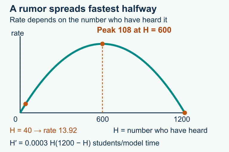The idealized rumor rate is greatest when half the 1200-person population has heard it; pictured students are qualitative context.

Question 5: CRITICAL THINKING

4 pts

A tank initially contains 100 liters of pure water. A brine solution with a salt concentration of 0.5 kg/L flows into the tank at a rate of 4 L/min. The well-mixed solution flows out at the same rate of 4 L/min. (a) Let S(t) be the amount of salt (in kg) in the tank at time t minutes. Explain why the rate of salt entering is 2 kg/min and write an expression for the rate of salt leaving. (b) Write a differential equation for dS/dt that models this situation and state the initial condition. (c) Identify the equilibrium solution and interpret it in context.

Show answer

Rubric (4 points): Point 1 (Part a — Rate In): Salt enters at (concentration in) × (flow rate in) = 0.5 kg/L × 4 L/min = 2 kg/min. The rate of salt leaving depends on the current concentration in the tank, which is S(t)/100 kg/L (since the volume remains constant at 100 L because inflow rate equals outflow rate). Thus, rate out = (S/100) × 4 = 4S/100 = S/25 kg/min. Point 2 (Part b — Differential Equation): dS/dt = (rate in) − (rate out) = 2 − S/25. The initial condition is S(0) = 0 (pure water initially). Point 3 (Part b — Recognizing Model Type): This can be rewritten as dS/dt = −(1/25)(S − 50), which has the form dy/dt = k(y − yₑ), a Newton's Cooling–type equation. The general structure is the same: the rate of change is proportional to the difference between the current amount and an equilibrium value. Point 4 (Part c — Equilibrium and Interpretation): Setting dS/dt = 0: 2 − S/25 = 0, so S = 50 kg. The equilibrium solution is S = 50. In context, this means that eventually the tank will contain 50 kg of salt, corresponding to a concentration of 50/100 = 0.5 kg/L—exactly the concentration of the incoming solution. This makes physical sense: when the tank concentration matches the inflow concentration, there is no net change in salt.

SUMMARY

Lesson Summary

Summary

Modeling with differential equations is the process of translating verbal descriptions of real-world change into precise mathematical statements. The key skill is recognizing verbal cues—phrases like "rate of change," "proportional to," and "difference between"—and converting them into derivatives and algebraic expressions. The three foundational models on the AP Calculus AB exam are exponential growth/decay (dy/dt = ky), logistic growth (dy/dt = ky(1 − y/L)), and Newton's Law of Cooling (dT/dt = k(T − Tₛ)). Each model has a characteristic solution shape—unbounded exponential, S-shaped logistic, or asymptotic approach to equilibrium.

An initial condition selects a unique particular solution from the family of solutions to a given differential equation. On the exam, you must be able to set up the correct DE from a word problem, verify that a given function solves a DE by substitution, and interpret equilibrium solutions (where dy/dt = 0) in context. For the logistic model, the maximum rate of change occurs at y = L/2. Remember: differential equations describe how a quantity changes, and solving them tells you what the quantity becomes over time.