

SECTION 1
Historical Context & Motivation
The idea that a smooth curve must, at some interior point, have a tangent line parallel to the line joining its endpoints feels intuitively obvious, yet it took centuries of mathematical development to articulate this principle rigorously. The Mean Value Theorem (MVT) sits at the heart of differential calculus because it provides the bridge between local information (derivatives at a point) and global behavior (change over an interval). Before the MVT was formalized, mathematicians relied on geometric intuition alone, which, while powerful, could not support the analytic machinery needed for proofs about monotonicity, concavity, and L'Hôpital's Rule. Understanding the historical arc of this theorem reveals why it remains indispensable on the AP Calculus AB exam and in every branch of analysis.
1691 • Rolle's Theorem Published
1797 • Lagrange's Formulation
1823 • Cauchy's Generalized MVT
1861 • Weierstrass's Rigor
The central question the MVT answers is deceptively simple: if a function is well-behaved on a closed interval, must there exist at least one interior point where the instantaneous rate of change matches the average rate of change over the entire interval? The theorem guarantees the answer is yes—and that guarantee is what powers many of the deeper results you will encounter in differential calculus.
SECTION 2
Core Principles & Definitions
Before applying the Mean Value Theorem, you must internalize its hypotheses and conclusion as separate, checkable conditions. The theorem is an existence result: it tells you a particular value c exists but does not tell you how to find it directly. Your job on the AP exam is to verify the hypotheses, invoke the theorem, and, when asked, solve for c. The following foundational ideas organize the entire framework.
Continuity on [a, b]
Differentiability on (a, b)
Existence of c
Rolle's Theorem as a Special Case
KEY TAKEAWAY
SECTION 3
Visual Explanation
The diagram below illustrates the geometric essence of the Mean Value Theorem. A smooth curve y = f(x) connects points A = (a, f(a)) and B = (b, f(b)). The secant line through A and B represents the average rate of change over [a, b]. The MVT guarantees at least one interior point c where the tangent line is parallel to that secant—that is, the slopes are equal.
Geometrically, the MVT asserts that you can always find at least one point on a smooth arc where the tangent line has the same slope as the chord connecting the arc's endpoints. If the curve dips and rises multiple times, there may be several such points c, but the theorem only requires the existence of at least one. When working exam problems, always verify the hypotheses first: a function that fails continuity at even one point of [a, b] or fails differentiability at an interior point may violate the theorem's conclusion.
 Continuity on the closed interval and differentiability in its interior guarantee a tangent parallel to the endpoint secant.
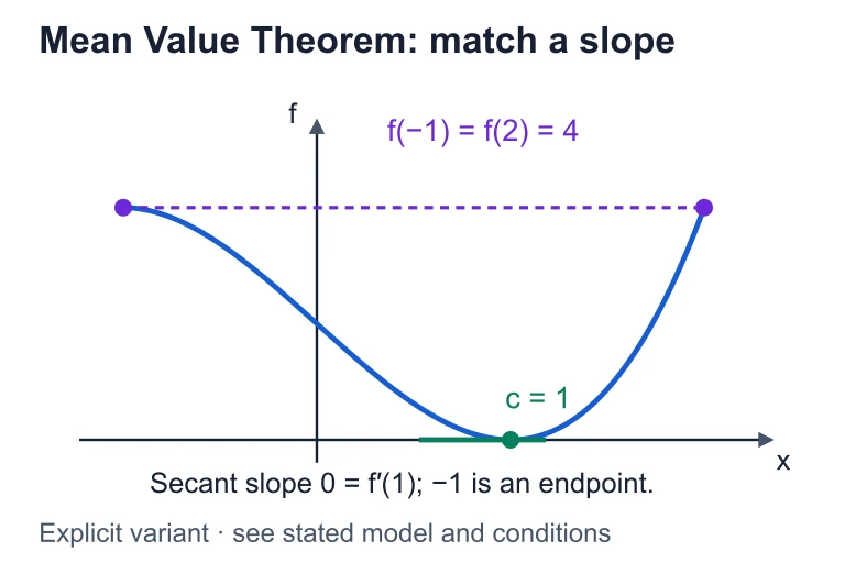 Continuity on the closed interval and differentiability in its interior guarantee a tangent parallel to the endpoint secant.
SECTION 4
Mathematical Framework
The formal statement of the MVT and its special case, Rolle's Theorem, are presented below with precise notation. Understanding the relationship between these two results is crucial because the proof of the MVT actually reduces to an application of Rolle's Theorem on an auxiliary function.
ROLLE'S THEOREM
This is the special case where the average rate of change is zero (the endpoints are at equal heights). The guaranteed point c is a local extremum.
MEAN VALUE THEOREM
Hypotheses: (1) f is continuous on [a, b], (2) f is differentiable on (a, b). Conclusion: there exists at least one c ∈ (a, b) satisfying the equation above, where the left side is the instantaneous rate of change at c and the right side is the average rate of change over the entire interval.
Proof Sketch via Rolle's Theorem
Define the auxiliary function g(x) = f(x) − [f(a) + ((f(b) − f(a))/(b − a)) × (x − a)]. The term subtracted from f(x) is the secant-line function, which is the equation of the straight line through (a, f(a)) and (b, f(b)). By construction, g(a) = 0 and g(b) = 0, so Rolle's Theorem applies to g. Therefore, there exists c ∈ (a, b) with g′(c) = 0. Computing g′(x) = f′(x) − (f(b) − f(a))/(b − a) and setting it to zero gives the MVT conclusion: f′(c) = (f(b) − f(a))/(b − a). This elegant reduction underscores that Rolle's Theorem and the MVT are essentially the same result viewed from different angles.
AUXILIARY FUNCTION
g measures the vertical distance between the curve and the secant line. Since g(a) = g(b) = 0, Rolle's Theorem guarantees g′(c) = 0 for some c in (a, b).
SECTION 5
Checking Hypotheses & Common Pitfalls
On the AP exam, a significant number of MVT questions test whether you can correctly verify—or identify the failure of—the theorem's hypotheses. The diagram below catalogs the three most common situations where the MVT cannot be applied, contrasted with a valid scenario. Developing fluency with these cases will prevent careless errors on both the multiple-choice and free-response sections.
Common Hypothesis-Check Strategies
- ✓ Polynomials are continuous and differentiable everywhere, so the MVT always applies on any closed interval.
- ✓ Rational functions require that the interval [a, b] contains no zeros of the denominator.
- ✓ Absolute value and piecewise functions may fail differentiability at the point where the formula changes; check the open interval (a, b) for corners.
- ✓ Square root and cube root functions may have vertical tangent lines (undefined derivatives) at endpoints; ensure such points are not in the open interval.
SECTION 6
Worked Example
Let us walk through a complete application of the MVT on a concrete function. This mirrors the style of free-response questions on the AP Calculus AB exam, where you must state hypotheses, apply the theorem, and solve for the guaranteed value of c.
Find c guaranteed by the MVT for f(x) = x³ − 3x + 2 on [−1, 2]
- 1
Step 1 — Verify Continuity
Since f(x) = x³ − 3x + 2 is a polynomial, it is continuous on all of ℝ and therefore continuous on the closed interval [−1, 2].✓ Continuity satisfied - 2
Step 2 — Verify Differentiability
Polynomials are differentiable everywhere, so f is differentiable on the open interval (−1, 2).✓ Differentiability satisfied - 3
Step 3 — Compute the Average Rate of Change
Evaluate f at the endpoints: f(−1) = (−1)³ − 3(−1) + 2 = −1 + 3 + 2 = 4 and f(2) = (2)³ − 3(2) + 2 = 8 − 6 + 2 = 4. The average rate of change is [f(2) − f(−1)] / (2 − (−1)) = (4 − 4) / 3 = 0.Average rate of change = 0 - 4
Step 4 — Set f′(c) Equal to the Average Rate
Differentiate: f′(x) = 3x² − 3. Set f′(c) = 0, giving 3c² − 3 = 0, so c² = 1, yielding c = ±1.c = −1 or c = 1 - 5
Step 5 — Select c in the Open Interval (−1, 2)
The value c = −1 is an endpoint, not in the open interval (−1, 2), so we discard it. The value c = 1 lies in (−1, 2) and satisfies the MVT conclusion. Note: because f(−1) = f(2), this is also an application of Rolle's Theorem.c = 1 ∈ (−1, 2) ✓
AP Exam Tip
SECTION 7
Strengths, Limitations & Related Theorems
The MVT is powerful but not omnipotent. Understanding its strengths alongside its limitations will deepen your problem-solving instinct and help you choose the right tool among several related theorems.
| Feature | Strength | Limitation |
|---|---|---|
| Existence guarantee | Guarantees at least one c where f′(c) equals the average rate—useful for proofs. | Does not specify how many such values c exist or how to find them without solving f′(c) = k. |
| Hypothesis requirements | Hypotheses are easy to verify for polynomials, trig, exponentials, and their compositions. | Fails for piecewise functions with corners, absolute value at the kink, or functions with asymptotes in the interval. |
| Applications | Proves the Increasing/Decreasing Test, justifies bounds on function values, and underlies L'Hôpital's Rule. | Cannot establish existence of maxima/minima directly; the Extreme Value Theorem is needed for that. |
| Specificity of c | For simple functions, c can be computed exactly. | For complex functions (e.g., f(x) = eˣ sin x), f′(c) = k may not have a closed-form solution. |
Strengths and limitations of the Mean Value Theorem
KEY TAKEAWAY
SECTION 8
Connection to Advanced Theory
The Mean Value Theorem is not an isolated result—it is the linchpin connecting basic differentiation to the deeper theorems of real analysis. On the AP exam, the MVT's consequences appear in justifications for increasing/decreasing behavior and in limit-based arguments. Beyond the AP curriculum, the MVT generalizes in several important directions that you may encounter in multivariable calculus and beyond.
| MVT (AP Calculus AB) | Advanced Extension |
|---|---|
| If f′(x) > 0 on (a, b), then f is increasing on [a, b]. | The Monotone Function Theorem in analysis formalizes this using the MVT as its proof engine. |
| If f′(x) = 0 for all x in (a, b), then f is constant on [a, b]. | The Zero Derivative Theorem, proved directly via the MVT, is essential in proving uniqueness of antiderivatives. |
| MVT applies to a single function f on a single interval. | Cauchy's Generalized MVT relates two functions f and g, producing f′(c)/g′(c) = [f(b)−f(a)]/[g(b)−g(a)], which is used to prove L'Hôpital's Rule. |
| One-variable MVT: f′(c) = Δf / Δx. | In multivariable calculus, the MVT extends to ∇f · (b − a) = f(b) − f(a) for vector-valued paths, connecting gradients to net change. |
From AP Calculus AB to advanced analysis
For your immediate AP preparation, the most critical consequence is the Increasing/Decreasing Test: if f′(x) > 0 for all x in an interval, then f is increasing there. This result is impossible to prove rigorously without the MVT, and you will invoke it every time you analyze the behavior of a function using its first derivative. Similarly, knowing that two functions with identical derivatives on an interval must differ by a constant (the constant difference theorem) is a direct consequence of the MVT and is foundational to the study of antiderivatives in Unit 6.
SECTION 9
Practice Problems
Question 1: CONCEPTUAL
- A. f′(c) = 3 for some c in (2, 5)
- B. f′(c) = 3 for some c in [2, 5]
- C. f′(x) = 3 for all x in (2, 5)
- D. f has a maximum at some c where f′(c) = 3
- E. f′(c) = 9 for some c in (2, 5)
Show answer (A)
Question 2: BASIC CALCULATION
- A. c = 1
- B. c = 2
- C. c = 3
- D. c = 5/2
- E. c = 3/2
Show answer (B)
Question 3: INTERMEDIATE
- A. c = 4
- B. c = 5
- C. c = 16/9
- D. c = 25/4
- E. c = 9/4
Show answer (A)
Question 4: APPLIED
5 ptsShow answer
Question 5: CRITICAL THINKING
3 ptsShow answer
SUMMARY
Lesson Summary
Summary
The Mean Value Theorem states that if f is continuous on [a, b] and differentiable on (a, b), then there exists at least one c in (a, b) where f′(c) = [f(b) − f(a)] / (b − a). Geometrically, this means the tangent line at c is parallel to the secant line connecting (a, f(a)) and (b, f(b)). Rolle's Theorem is the special case where f(a) = f(b), yielding f′(c) = 0.
To apply the MVT on the AP exam: (1) verify both hypotheses explicitly, (2) compute the average rate of change, (3) set f′(c) equal to that value and solve, and (4) confirm c lies in the open interval (a, b). The MVT underpins the Increasing/Decreasing Test, the Constant Difference Theorem, and serves as the foundation for L'Hôpital's Rule via Cauchy's generalization.