Introduction to Optimization Problems - AP Calculus AB

SECTION 1

Historical Context & Motivation

The desire to find the best possible outcome—whether maximizing profit, minimizing cost, or enclosing the greatest area—predates calculus itself. Ancient Greek mathematicians recognized that among all plane figures with a given perimeter, the circle encloses the greatest area, a result known as the isoperimetric inequality. However, without a systematic method for locating extrema, these early insights relied on geometric ingenuity rather than general algorithms. The invention of calculus in the seventeenth century transformed optimization from a collection of clever tricks into a powerful, unified framework applicable across mathematics, physics, economics, and engineering.

~300 BCE • Euclid & the Greeks

Greek geometers established that a square maximizes the area of a rectangle with fixed perimeter, using purely geometric arguments without calculus.

1629 • Fermat's Method of Adequality

Pierre de Fermat developed a proto-derivative technique called adequality, allowing him to find tangent lines and locate maxima and minima of polynomial expressions.

1684–1687 • Newton & Leibniz Formalize Calculus

Isaac Newton and Gottfried Wilhelm Leibniz independently published the fundamental rules of differentiation, providing the systematic machinery for optimization.

1696 • The Brachistochrone Problem

Johann Bernoulli challenged Europe's mathematicians to find the curve of fastest descent, sparking the development of the calculus of variations—optimization extended to functions.

Modern Era • Optimization in Science & Industry

Today, calculus-based optimization underpins machine learning, operations research, structural engineering, and economic modeling, making it one of the most widely applied branches of mathematics.

The central question that optimization addresses is deceptively simple: given a quantity that depends on one or more variables, what value of those variables makes the quantity as large or as small as possible? In AP Calculus AB, you will focus on single-variable optimization—problems in which a real-valued function of one variable must be maximized or minimized over a given domain. The key insight is that derivatives encode the rate of change, so setting the derivative equal to zero identifies candidate points where the function transitions from increasing to decreasing (or vice versa).

SECTION 2

Core Principles of Optimization

Every optimization problem in AP Calculus AB rests on a handful of foundational principles. Understanding these principles before diving into specific problems will give you a reliable framework that applies whether you are maximizing revenue, minimizing surface area, or finding the shortest distance. The interplay between derivatives, critical points, and domain constraints forms the backbone of the technique.

Objective Function

The quantity you want to optimize must be expressed as a function of a single variable, f(x). Translating a word problem into this function is typically the most challenging step.

Constraint Equation

Most real-world problems impose a constraint (e.g., fixed perimeter, limited material). Use the constraint to eliminate one variable so that your objective function depends on only one variable.

Feasible Domain

Physical or geometric restrictions limit the variable to a specific interval. Identifying this domain is essential because the Extreme Value Theorem guarantees an absolute extremum on a closed interval.

Critical Points

Set f ′(x) = 0 or identify where f ′(x) is undefined within the domain. These critical points, together with the endpoints of the domain, are the only candidates for absolute extrema.

Verification

Use the Closed Interval Test (compare function values at critical points and endpoints), the First Derivative Test, or the Second Derivative Test to confirm whether a candidate is a maximum or minimum.

✦

KEY TAKEAWAY

Think of optimization like tuning a radio: you sweep through frequencies (the domain) and listen for the strongest signal (maximum of f). The derivative tells you whether the signal is getting stronger or weaker, and a critical point is where the signal stops improving—potentially the clearest reception you can find.

SECTION 3

Visual Explanation: Anatomy of an Optimization Problem

The diagram below illustrates a generic optimization scenario on a closed interval [a, b]. The objective function f(x) is plotted along with its derivative f ′(x). Observe how the critical points occur precisely where f ′(x) = 0, and the absolute maximum and minimum are identified by comparing function values at these critical points and at the endpoints of the interval.

The curve f(x) has three critical points c₁, c₂, and c₃ where f ′(x) = 0. Comparing f(a), f(c₁), f(c₂), f(c₃), and f(b) reveals that c₃ yields the absolute maximum on [a, b]. This comparison process is the Closed Interval Test.

Notice that the absolute maximum does not have to occur at an endpoint. It occurs at c₃, a critical point in the interior of the interval. Similarly, the absolute minimum on this interval is at the endpoint a, which reinforces why you must always evaluate f at both endpoints and all critical points before drawing conclusions.

SECTION 4

Mathematical Framework

The mathematical backbone of optimization problems consists of three theorems and a systematic procedure for applying them. Mastering this framework ensures that you approach every optimization problem with a clear, repeatable strategy.

EXTREME VALUE THEOREM

If f is continuous on [a, b], then f attains an absolute maximum M and an absolute minimum m on [a, b].

This theorem guarantees that a solution exists, provided the function is continuous and the domain is a closed interval. Always verify these conditions before proceeding.

FIRST DERIVATIVE TEST FOR ABSOLUTE EXTREMA

If f ′(x) changes from positive to negative at x = c, then f(c) is a local maximum. If f ′(x) changes from negative to positive, then f(c) is a local minimum.

On an open interval or when you need to confirm the nature of a single critical point, the sign change of f ′ around c is decisive.

SECOND DERIVATIVE TEST

If f ′(c) = 0 and f ″(c) > 0, then f(c) is a local minimum. If f ′(c) = 0 and f ″(c) < 0, then f(c) is a local maximum.

When f ″(c) = 0, the test is inconclusive; fall back on the First Derivative Test or the Closed Interval Test.

CLOSED INTERVAL TEST

Evaluate f at each critical point c in (a, b) and at the endpoints a and b. The largest value is the absolute maximum; the smallest is the absolute minimum.

This brute-force comparison is the most reliable method when the domain is a closed interval.

Optimization Problem-Solving Procedure

Draw a diagram and label all quantities. Assign variables to the unknowns.
Write the objective function—the quantity to be maximized or minimized—in terms of the variables.
Use the constraint to eliminate all but one variable so that the objective function becomes f(x).
Determine the feasible domain of x based on physical or geometric restrictions.
Differentiate f(x), set f ′(x) = 0, and solve for critical points.
Verify using the Closed Interval Test, the First Derivative Test, or the Second Derivative Test.
Answer the question—state both the optimal value of the variable and the optimal value of the objective function, including appropriate units.

SECTION 5

Common Optimization Problem Types

AP Calculus AB optimization problems fall into several recurring categories. Recognizing the type of problem you face helps you set up the objective function and constraint equation more quickly. The diagram below classifies the most common scenarios you will encounter, along with their typical constraint and objective structures.

The three most common optimization categories on the AP exam—geometric, distance/rate, and economic—all follow the same six-step strategy outlined at the bottom of the diagram.

Problem Type	Typical Objective	Typical Constraint	Key Tip
Fenced Area	Maximize A = xy	Fixed perimeter or fencing length	If one side is a wall, perimeter equation changes
Open-Top Box	Maximize V = x²h or V = lwh	Sheet dimensions fix l, w in terms of cut size x	Domain: 0 < x < half of the shorter side
Min Distance	Minimize D² = (x − a)² + (y − b)²	Point (x, y) lies on a given curve	Minimize D² to avoid the square root
Min Surface Area	Minimize S = 2πr² + 2πrh	Fixed volume V = πr²h	Solve constraint for h, substitute into S
Revenue / Profit	Maximize R(x) = x · p(x)	Demand function p(x) given	Profit = Revenue − Cost

Summary of common AP Calculus AB optimization problem archetypes

A cardboard net with four corner squares removed, partly folded walls, and a finished open-top box on a worktable. Suppose an open box is made from a 12 cm square sheet. Cutting corners of side x gives V(x) = x(12 − 2x)² for 0 < x < 6; the maximum is 128 cm³ at x = 2 cm.

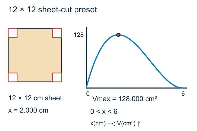Suppose an open box is made from a 12 cm square sheet. Cutting corners of side x gives V(x) = x(12 − 2x)² for 0 < x < 6; the maximum is 128 cm³ at x = 2 cm.

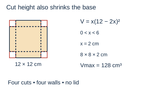A 12 cm square net has four equal corner cuts and dashed fold lines, with the resulting 8 × 8 × 2 cm box and volume 128 cm³. Cutting 2 cm squares from each corner of a 12 cm square sheet leaves an 8 × 8 cm base and 2 cm walls. The resulting volume 128 cm³ is the maximum of V(x) = x(12 − 2 x)² on 0 < x < 6.Open full diagram

SECTION 6

Worked Example: Maximizing the Area of a Fenced Region

A farmer has 120 meters of fencing and wants to enclose a rectangular garden against a straight river (no fencing is needed along the river). What dimensions maximize the enclosed area?

Maximizing Area with a River Boundary

1
Step 1 — Draw a Diagram and Define Variables

Let x be the length of the side parallel to the river and y be the length of each of the two sides perpendicular to the river. The river forms the fourth side, so no fencing is needed there.
2
Step 2 — Write the Objective Function

The area of the rectangle is A = xy. This is the quantity we want to maximize.

A = xy
3
Step 3 — Write the Constraint and Eliminate a Variable

The total fencing used is x + 2y = 120. Solving for x gives x = 120 − 2y. Substituting into the area function yields A(y) = (120 − 2y)y = 120y − 2y².

A(y) = 120y − 2y²
4
Step 4 — Determine the Feasible Domain

Since y represents a physical length, y > 0. Also, x = 120 − 2y must be positive, so y < 60. The feasible domain is 0 < y < 60, or we can consider the closed interval [0, 60] where A = 0 at both endpoints.

Domain: 0 ≤ y ≤ 60
5
Step 5 — Differentiate and Find Critical Points

A′(y) = 120 − 4y. Setting A′(y) = 0: 120 − 4y = 0, so y = 30.

Critical point: y = 30
6
Step 6 — Verify It Is a Maximum

A″(y) = −4, which is negative for all y, so by the Second Derivative Test, y = 30 yields a local (and global) maximum. Alternatively, A(0) = 0, A(30) = 1800, A(60) = 0, confirming y = 30 gives the absolute maximum by the Closed Interval Test.

A″(30) = −4 < 0 → Maximum confirmed
7
Step 7 — State the Answer

When y = 30 m, x = 120 − 2(30) = 60 m. The maximum enclosed area is A = 60 × 30 = 1800 m².

Maximum area = 1800 m² when x = 60 m and y = 30 m

💡

AP Exam Tip

On the free-response section, always justify that your critical point yields a maximum (or minimum), not just an extremum. State which test you used—Second Derivative Test or Closed Interval Test—and show the supporting computation. Without justification, you will lose rubric points even if your numerical answer is correct.

Selected v2 has one landscape, three fence runs and an unfenced river edge; generated graph and duplicate inset were removed. With the river side unfenced, 120 m of fencing gives x + 2y = 120. The largest rectangular area is 1,800 m², with x = 60 m and y = 30 m.

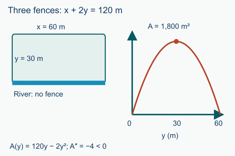With the river side unfenced, 120 m of fencing gives x + 2y = 120. The largest rectangular area is 1,800 m², with x = 60 m and y = 30 m.

SECTION 7

Common Mistakes & How to Avoid Them

Optimization problems are multi-step, and errors can creep in at any stage—from misidentifying the objective function to neglecting domain restrictions. The table below catalogs the most frequent mistakes students make on the AP exam, along with strategies for avoiding each one.

Common Mistake	Why It's Wrong	Correct Approach
Leaving two variables in the objective function	You cannot differentiate with respect to x if y is still present as an independent variable	Always use the constraint to eliminate one variable before differentiating
Ignoring the domain	A critical point outside the feasible domain is irrelevant; negative lengths are meaningless	Write the domain explicitly before differentiating; check that every critical point lies within it
Forgetting to check endpoints	On a closed interval, absolute extrema may occur at endpoints, not at critical points	Evaluate f at all critical points and both endpoints; compare all values
Not justifying max vs. min	Finding f ′(c) = 0 does not guarantee a maximum—it could be a minimum or neither	Explicitly state and apply the Second Derivative Test or First Derivative Test
Answering the wrong question	The problem may ask for the dimensions, not the area; or the minimum cost, not the dimensions	Re-read the question after solving; provide exactly what is requested

Common optimization pitfalls on the AP Calculus AB exam

✦

KEY TAKEAWAY

Think of the optimization procedure as an engineering checklist before a rocket launch: skipping even one step—like verifying the domain or justifying the nature of the critical point—can cause the entire solution to fail. Systematic rigor, not speed, is what earns full credit on the AP exam.

SECTION 8

Connection to Advanced Topics

The single-variable optimization techniques you learn in AP Calculus AB form the foundation for far more powerful methods encountered in higher mathematics. Understanding where single-variable optimization fits in the broader landscape will deepen your conceptual grasp and prepare you for future coursework in multivariable calculus, differential equations, and applied mathematics.

Feature	AP Calculus AB (Single-Variable)	Advanced (Multivariable / Constrained)
Number of variables	One independent variable after substitution	Two or more independent variables simultaneously
Handling constraints	Substitute constraint to eliminate a variable	Lagrange multipliers handle constraints without elimination
Critical point condition	f ′(x) = 0	∇f = 0 (gradient equals the zero vector)
Second-order test	f ″(c) > 0 or f ″(c) < 0	Hessian matrix eigenvalue analysis
Domain	Interval on the real line	Region in ℝⁿ (bounded by surfaces or inequalities)

Single-variable vs. multivariable optimization

In AP Calculus BC and beyond, you will encounter problems where it is not practical to eliminate variables through substitution—for instance, optimizing a function of three variables subject to two constraints. Lagrange multipliers provide an elegant alternative: rather than eliminating variables, you introduce a new unknown (the multiplier λ) and solve a system of equations that simultaneously satisfies the optimality and constraint conditions. The intuition behind Lagrange multipliers—that at an extremum the gradient of the objective function is parallel to the gradient of the constraint—builds directly on the idea that f ′(x) = 0 at a critical point. Everything you master now in single-variable optimization extends naturally into these richer settings.

SECTION 9

Practice Problems

Question 1: CONCEPTUAL

A continuous function f is defined on the closed interval [−3, 5]. The function has exactly one critical point at x = 1, where f ′(1) = 0. Which of the following must be true?

A. f(1) is the absolute maximum of f on [−3, 5].
B. f(1) is either a local maximum or a local minimum.
C. The absolute maximum of f on [−3, 5] occurs at x = −3, x = 1, or x = 5.
D. f has an inflection point at x = 1.
E. f ″(1) < 0.

Show answer (C)

Answer: C. By the Extreme Value Theorem, a continuous function on a closed interval attains its absolute maximum and minimum. The candidates for the absolute maximum are the endpoints and all critical points in the interior. Since x = 1 is the only critical point, the absolute maximum must occur at x = −3, x = 1, or x = 5. (A) is wrong because the maximum could occur at an endpoint, not necessarily at x = 1. (B) is wrong because f ′(1) = 0 does not guarantee a local extremum—the point could be an inflection point with a horizontal tangent, as in f(x) = x³ at x = 0. (D) is wrong because f ′(c) = 0 does not imply an inflection point. (E) is wrong because no information about f ″ is given.

Question 2: BASIC CALCULATION

A rectangle has a perimeter of 40 cm. What is the maximum possible area of the rectangle?

A. 80 cm²
B. 100 cm²
C. 120 cm²
D. 160 cm²
E. 200 cm²

Show answer (B)

Answer: B. Let the sides be x and y. The constraint is 2x + 2y = 40, so y = 20 − x. The area function is A(x) = x(20 − x) = 20x − x² on the domain [0, 20]. Differentiating: A′(x) = 20 − 2x = 0 gives x = 10. Then y = 10 and A = 100 cm². Since A″(x) = −2 < 0, this is indeed a maximum. (A) 80 corresponds to a 4 × 16 rectangle; (C) 120, (D) 160, and (E) 200 exceed the geometric maximum possible for this perimeter.

Question 3: INTERMEDIATE

An open-top rectangular box is to be made from a 12 cm × 12 cm sheet of cardboard by cutting equal squares of side length x from each corner and folding up the sides. Find the value of x that maximizes the volume of the box, and state the maximum volume.

A. x = 2 cm, V = 128 cm³
B. x = 3 cm, V = 108 cm³
C. x = 4 cm, V = 64 cm³
D. x = 1 cm, V = 100 cm³
E. x = 2.5 cm, V = 122.5 cm³

Show answer (A)

Answer: A. After cutting squares of side x from each corner, the base has dimensions (12 − 2x) × (12 − 2x) and the height is x. So V(x) = x(12 − 2x)² on the domain 0 < x < 6. Expanding: V(x) = x(144 − 48x + 4x²) = 4x³ − 48x² + 144x. Then V′(x) = 12x² − 96x + 144 = 12(x² − 8x + 12) = 12(x − 2)(x − 6). Setting V′(x) = 0 gives x = 2 or x = 6. Since x = 6 is an endpoint where V = 0, x = 2 is the only viable critical point. V(2) = 2(8)² = 128 cm³. V″(x) = 24x − 96, so V″(2) = −48 < 0, confirming a maximum. (B) uses x = 3 incorrectly: V(3) = 3(6)² = 108 < 128. (C), (D), and (E) yield smaller volumes.

Question 4: APPLIED

5 pts

A manufacturer produces cylindrical cans that must hold exactly 500 cm³ of liquid. The material for the top and bottom costs $0.04 per cm², and the material for the curved side costs $0.02 per cm². (a) Express the total cost C as a function of the radius r. (b) Find the radius r that minimizes the total cost. (c) Find the corresponding height h. (d) Justify that your answer gives a minimum.

Show answer

Rubric (5 points): Point 1 — Setting up the cost function: The top and bottom each have area πr², costing 0.04(2πr²) = 0.08πr². The lateral surface has area 2πrh, costing 0.02(2πrh) = 0.04πrh. Total cost: C = 0.08πr² + 0.04πrh. Point 2 — Eliminating h using the volume constraint: From V = πr²h = 500, we get h = 500/(πr²). Substituting: C(r) = 0.08πr² + 0.04πr · 500/(πr²) = 0.08πr² + 20/r, for r > 0. Point 3 — Finding the critical point: C′(r) = 0.16πr − 20/r². Setting C′(r) = 0: 0.16πr = 20/r², so r³ = 20/(0.16π) = 125/π, giving r =

(125/π)^{1/3}

≈ 3.414 cm. Point 4 — Finding the corresponding height: h = 500/(πr²) = 500/(π

(125/π)^{2/3}

). This simplifies to h ≈ 13.66 cm. Point 5 — Justification that this is a minimum: C″(r) = 0.16π + 40/r³. Since both terms are positive for all r > 0, C″(r) > 0 for all r in the domain. In particular, C″ at the critical point is positive, so the Second Derivative Test confirms a local minimum. Since this is the only critical point on (0, ∞) and C → ∞ as r → 0⁺ and as r → ∞, it is also the absolute minimum. Cost C(r)=0.08πr²+20/r for a closed cylinder of volume 500 cm³. The minimum occurs at r about 3.414 cm, with h=4r.

Cost C(r)=0.08πr²+20/r for a closed cylinder of volume 500 cm³. The minimum occurs at r about 3.414 cm, with h=4r.

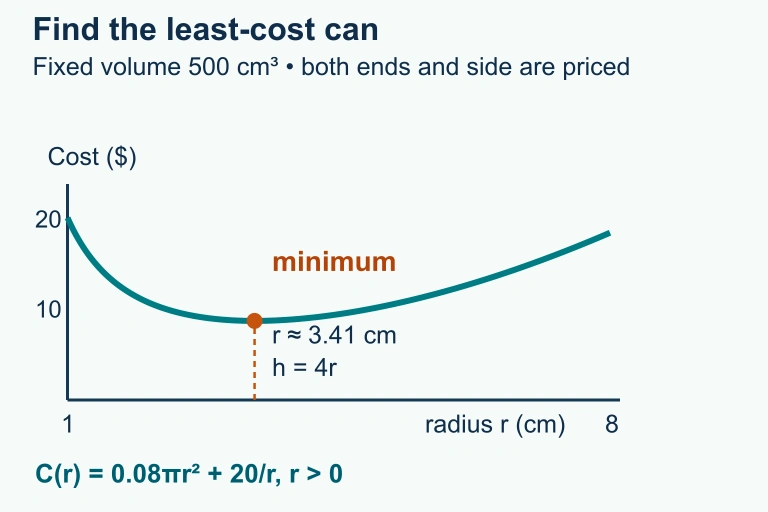At fixed 500 cm³ volume and the stated unequal material costs, the least-cost closed can has h=4 r.

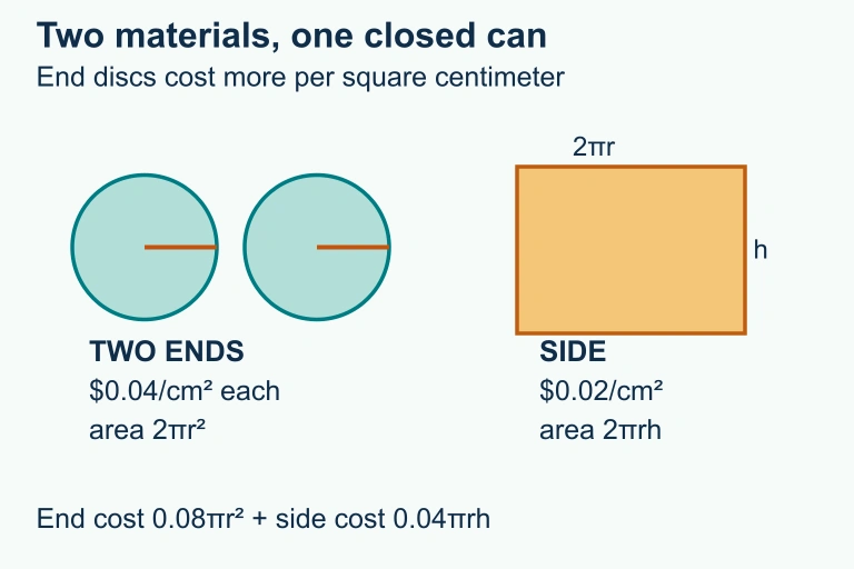A cylinder separated into two circular ends priced at 0.04 per cm² and a side rectangle priced at 0.02 per cm². The rectangle has dimensions 2πr by h.

Question 5: CRITICAL THINKING

3 pts

A point P lies on the parabola y = x² in the first quadrant. A line segment connects the origin O = (0, 0) to P = (x, x²), and a second line segment connects P to the point Q = (4, 0) on the x-axis. (a) Express the total length L = OP + PQ as a function of x for x > 0. (b) Use calculus to find the value of x that minimizes L. Justify your answer. (c) Explain why minimizing L² would not be a valid simplification in this problem, even though minimizing D² is valid when minimizing a single distance.

Show answer

Rubric (3 points): Point 1 — Writing L(x): OP = √(x² + x⁴) = x√(1 + x²) (since x > 0). PQ = √((x − 4)² + x⁴). Therefore L(x) = x√(1 + x²) + √((x − 4)² + x⁴). Point 2 — Finding the minimum and justification: Set L′(x) = 0 and solve (this requires a calculator). L′(x) = d/dx[x√(1 + x²)] + d/dx[√((x − 4)² + x⁴)]. Using the chain rule: the first term's derivative is (1 + 2x²)/√(1 + x²), and the second term's derivative is [(x − 4) + 2x³] / √((x − 4)² + x⁴). Setting the sum equal to zero and solving numerically yields x ≈ 0.890. Since L(x) → ∞ as x → 0⁺ and as x → ∞, and there is a single critical point in (0, ∞), this critical point gives the absolute minimum by the behavior of L at the boundary of the domain. Point 3 — Explaining why minimizing L² fails: The trick of minimizing D² instead of D works because D² = f(x) is a composition with a strictly increasing function (squaring), so the minimum of D² occurs at the same x as the minimum of D. However, L is a sum of two square roots: L = D₁ + D₂. The function L² = (D₁ + D₂)² = D₁² + 2D₁D₂ + D₂² contains a cross term 2D₁D₂ that depends on both distances simultaneously. Setting d(L²)/dx = 0 still finds the critical points of L² (which coincide with those of L), but the algebraic simplification that makes squaring useful—elimination of the square root—does not occur because the cross term reintroduces the radicals. Thus, squaring does not simplify the computation.

SUMMARY

Summary

Optimization problems ask you to find the absolute maximum or minimum of a quantity by applying the tools of differentiation. Every optimization problem follows a consistent procedure: identify the objective function (what you want to optimize), use the constraint equation to reduce the problem to a single variable, determine the feasible domain, find critical points by setting f ′(x) = 0, and then verify your answer using the Closed Interval Test, the First Derivative Test, or the Second Derivative Test.

The most common problem types on the AP exam include geometric optimization (maximizing area, minimizing surface area), distance minimization, and economic optimization (maximizing revenue or profit). Remember that the Extreme Value Theorem guarantees the existence of absolute extrema on a closed interval, so always check endpoints and critical points. On the free-response section, explicitly justify whether your critical point yields a maximum or minimum—this justification is required for full credit.