Introducing Calculus: Can Change Occur at an Instant? - AP Calculus AB

SECTION 1

Historical Context & Motivation

The question of whether change can be meaningfully described at a single instant is one of the oldest puzzles in mathematics and philosophy. Ancient Greek thinkers recognized that motion implies change over time, yet everyday experience insists that a speeding arrow possesses a definite velocity at each moment. This tension — between a process that unfolds over intervals and a quantity we wish to pin down at a point — drove millennia of debate before the invention of calculus finally provided rigorous tools to resolve it. Understanding this history illuminates why limits, rather than simple division, are the gateway to differential calculus.

~450 BCE • Zeno's Paradoxes

Zeno of Elea proposed paradoxes such as the Arrow Paradox, arguing that at any single instant an arrow occupies a fixed position and therefore cannot be moving — challenging the very idea of instantaneous motion.

~1670 • Newton & Leibniz Develop Calculus

Isaac Newton and Gottfried Wilhelm Leibniz independently created the foundational ideas of calculus. Newton's fluxions and Leibniz's differential notation gave the first systematic methods for computing instantaneous rates of change.

1821 • Cauchy Formalizes Limits

Augustin-Louis Cauchy introduced the modern epsilon-delta definition of a limit, replacing intuitive notions of 'infinitely small' quantities with a precise logical framework.

1861 • Weierstrass Completes Rigorization

Karl Weierstrass refined the epsilon-delta definition to its modern form, eliminating reliance on geometric intuition and establishing the analytical foundations that underpin every AP Calculus course today.

The central question this lesson addresses is deceptively simple: if rate of change is defined as the ratio of a change in output to a change in input, what happens when that change in input shrinks to zero? Direct substitution yields the indeterminate form 0 ÷ 0, which is meaningless. The concept of the limit resolves this by asking not what the ratio equals at zero, but what value it approaches as the interval becomes arbitrarily small. This idea is the philosophical and mathematical foundation of all of calculus.

SECTION 2

Core Principles & Definitions

Before we can rigorously define instantaneous rate of change, we need to establish a constellation of foundational ideas that connect the familiar concept of average rate of change to the new concept of a limit. These principles form the conceptual scaffolding for the entire AP Calculus AB curriculum, and mastering them here will make every subsequent topic — derivatives, integrals, and the Fundamental Theorem — far more intuitive.

Average Rate of Change

For a function f on the interval [a, b], the average rate of change is the slope of the secant line: (f(b) − f(a)) / (b − a). This requires two distinct points.

Instantaneous Rate of Change

The rate of change at a single point x = a, obtained by taking the limit of the average rate as the interval width h → 0. This is the slope of the tangent line.

The Limit

The value that a function's output approaches as the input approaches some target value. The limit need not equal the function's value at that point — it describes the trend, not the destination.

Secant → Tangent Transition

As the second point of a secant line slides closer to the fixed point, the secant line rotates toward the tangent line. The limiting position of the secant is the tangent.

Indeterminate Forms

Expressions like 0/0 are not undefined in the usual sense — they are indeterminate, meaning more analysis (a limit) is needed to find the actual value the expression approaches.

✦

KEY TAKEAWAY

Think of a GPS tracking a car's speed. The GPS doesn't measure speed at a literal instant — it computes distance traveled over very small time intervals and reports the result. As the interval shrinks, the reading converges on the car's true instantaneous speed. A limit is the mathematical version of this process: it captures what a ratio settles toward as the interval collapses, even though you can never actually divide by zero.

SECTION 3

Visual Explanation: Secant Lines Approach the Tangent

The diagram below illustrates the central geometric idea of this lesson. A smooth curve y = f(x) is shown with a fixed point A and several positions of a second point B. Each position of B determines a different secant line through A and B, and as B slides toward A along the curve, these secant lines rotate toward a single limiting position: the tangent line at A. The slope of this tangent line is the instantaneous rate of change of f at that point.

Point A (cyan) is fixed on the curve. The dashed secant lines pass through A and successive positions B₁, B₂, B₃, B₄ that move closer to A. The solid violet line is the tangent line — the limiting position of the secant — whose slope equals the instantaneous rate of change at A.

Notice that no single secant line equals the tangent line — the tangent is never actually reached by any secant because that would require B to coincide exactly with A, collapsing the two-point construction. Instead, the tangent is the limit of the family of secant lines. This is a geometric preview of the analytic definition you will formalize in the next section: the derivative of f at x = a is the limit of the difference quotient as the interval width approaches zero.

SECTION 4

Mathematical Framework

We now translate the geometric intuition of converging secant lines into precise algebraic language. The key quantity is the difference quotient, which measures the average rate of change of a function f over an interval of width h. Taking the limit of this quotient as h → 0 produces the instantaneous rate of change, provided the limit exists.

AVERAGE RATE OF CHANGE

Average Rate = [f(a + h) − f(a)] / h

Here a is the fixed input value, h is the interval width (h ≠ 0), and f(a + h) − f(a) is the change in output. This is the slope of the secant line through (a, f(a)) and (a + h, f(a + h)).

INSTANTANEOUS RATE OF CHANGE (THE DERIVATIVE)

f ′(a) = lim [f(a + h) − f(a)] / h as h → 0

The expression lim as h → 0 means we examine what happens to the difference quotient as h gets arbitrarily close to zero — without ever setting h = 0. If this limit exists and is finite, f is differentiable at x = a, and f ′(a) is the slope of the tangent line there.

ALTERNATIVE FORM (TWO-POINT NOTATION)

f ′(a) = lim [f(x) − f(a)] / (x − a) as x → a

This is algebraically equivalent. Here the variable point is x (rather than a + h), and the interval width is x − a. As x → a, the secant through (a, f(a)) and (x, f(x)) converges to the tangent at a.

A crucial subtlety: you cannot simply substitute h = 0 into the difference quotient because that would produce 0/0, which is algebraically undefined. The power of the limit is that it defines the instantaneous rate of change as the number that the difference quotient approaches, sidestepping the impossibility of dividing by zero. This is the resolution to Zeno's Arrow Paradox — calculus does not require you to freeze time; it requires you to analyze what happens in the neighborhood of an instant, using the limit as the bridge from finite intervals to a point.

💡

AP Exam Note

The College Board expects you to interpret limits of difference quotients in context. If a problem gives a table of values for a function s(t) representing position, you should be able to estimate the instantaneous velocity at a particular time by computing difference quotients over smaller and smaller intervals and identifying the value they approach.

SECTION 5

Detailed Breakdown: Approaching the Limit Numerically

One of the most effective ways to build intuition about limits is to compute the difference quotient for progressively smaller values of h and observe how the results converge. The following diagram and table illustrate this process for a specific function, showing how numerical evidence can suggest the value of an instantaneous rate of change before any algebraic simplification is performed.

For f(x) = x², the difference quotient at a = 3 approaches 6 from both sides as h → 0. This confirms that the instantaneous rate of change of x² at x = 3 is 6 — the slope of the tangent line to the parabola at that point.

The table confirms that as h shrinks toward zero from the positive side (right-hand approach), the difference quotient decreases toward 6: values of 7, 6.5, 6.1, 6.01, 6.001, and so on. Simultaneously, as h approaches zero from the negative side (left-hand approach), the quotient increases toward 6: values of 5.9, 5.99, and so on. Because both one-sided approaches agree, we conclude that the limit exists and equals 6. This numerical method is powerful for estimation, but algebraic confirmation (expanding and canceling) provides the exact answer and reveals why the limit works.

⚠

Why Both Sides Matter

For a limit to exist, the function must approach the same value from both directions. If the left-hand limit and the right-hand limit disagree, the two-sided limit does not exist. On the AP exam, checking both sides is essential when analyzing limits from tables or graphs.

SECTION 6

Worked Example: Finding Instantaneous Velocity

Suppose a ball is dropped from a tall building and its height (in meters) above the ground at time t seconds is modeled by s(t) = 100 − 4.9t². We want to find the instantaneous velocity of the ball at t = 2 seconds. Since velocity is the rate of change of position with respect to time, we need to compute the limit of the difference quotient of s at t = 2.

Finding the Instantaneous Velocity at t = 2

1
Step 1 — Set Up the Difference Quotient

Using the limit definition, the instantaneous velocity at t = 2 is v(2) = lim as h → 0 of [s(2 + h) − s(2)] / h. First, compute s(2): s(2) = 100 − 4.9(2)² = 100 − 4.9(4) = 100 − 19.6 = 80.4 meters.

s(2) = 80.4 m
2
Step 2 — Compute s(2 + h)

Expand s(2 + h) = 100 − 4.9(2 + h)² = 100 − 4.9(4 + 4h + h²) = 100 − 19.6 − 19.6h − 4.9h² = 80.4 − 19.6h − 4.9h².

s(2 + h) = 80.4 − 19.6h − 4.9h²
3
Step 3 — Form and Simplify the Quotient

Substitute into the difference quotient: [s(2 + h) − s(2)] / h = [(80.4 − 19.6h − 4.9h²) − 80.4] / h = (−19.6h − 4.9h²) / h. Factor h from the numerator: h(−19.6 − 4.9h) / h = −19.6 − 4.9h, valid for h ≠ 0.

Simplified quotient = −19.6 − 4.9h
4
Step 4 — Take the Limit as h → 0

Now take the limit: lim (h → 0) [−19.6 − 4.9h] = −19.6 − 4.9(0) = −19.6. The negative sign indicates the ball is moving downward.

v(2) = −19.6 m/s
5
Step 5 — Interpret the Result

At exactly t = 2 seconds, the ball is falling at a speed of 19.6 meters per second (downward). This is the instantaneous velocity — a quantity that exists at a single moment, not over an interval. The limit process transformed an average rate (over an interval of width h) into a precise rate at the instant t = 2.

💡

WHY THIS WORKS

The algebraic trick — expanding the expression and then canceling the common factor of h — is what eliminates the 0/0 indeterminate form. After cancellation, the remaining expression is a simple polynomial in h, and evaluating it at h = 0 is straightforward. This pattern (expand, cancel, evaluate) will recur throughout your study of derivatives.

One orange ball falls within a museum drop tower beside a computed height-time curve,tangent and signed velocity/speed readouts. For height s(t) = 100 − 4.9t² meters, equal time intervals produce increasingly large drops. The model ends at ground impact, about 4.52 seconds.

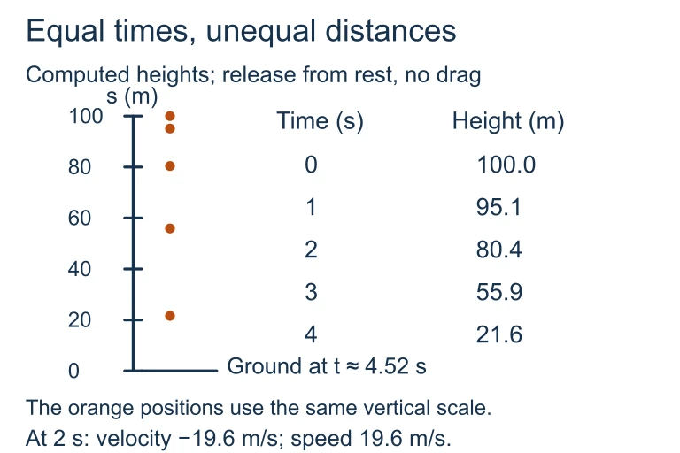For height s(t) = 100 − 4.9t² meters, equal time intervals produce increasingly large drops. The model ends at ground impact, about 4.52 seconds.

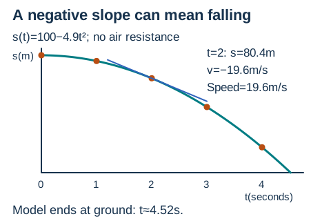A decreasing height-time curve ends at ground impact around 4.52 seconds. At 2 seconds, a tangent touches the point at 80.4 m with slope −19.6 m/s. For s(t) = 100 − 4.9 t² meters, the point at t = 2 seconds has height 80.4 m and tangent slope −19.6 m/s. The negative velocity means downward motion; speed is 19.6 m/s.Open full diagram

SECTION 7

Average vs. Instantaneous Rate of Change

A persistent source of confusion for students entering calculus is the distinction between average and instantaneous rates of change. While both describe how a quantity varies, they answer fundamentally different questions and are computed in fundamentally different ways. The table below clarifies the comparison across several dimensions.

Feature	Average Rate of Change	Instantaneous Rate of Change
Definition	[f(b) − f(a)] / (b − a)	lim (h→0) [f(a+h)−f(a)] / h
Geometric Meaning	Slope of the secant line through two points on the graph	Slope of the tangent line at a single point on the graph
Requires	Two distinct input values a and b	A limit process (infinitely many shrinking intervals)
Example (velocity)	Total distance ÷ total time over a trip	Reading on the speedometer at a specific moment
Notation	Δy / Δx	dy/dx or f ′(x)
AP Exam Context	Often computed from tables or used to estimate derivatives	The central object of differential calculus; appears in every FRQ

Comparison of average and instantaneous rates of change

🔑

THE BIG PICTURE

Average rate of change is algebra; instantaneous rate of change is calculus. The entire conceptual leap from precalculus to calculus is captured in the transition from Δy/Δx to dy/dx — from a finite ratio to a limit of ratios. Master this transition and the rest of calculus becomes a natural extension.

SECTION 8

Connection to the Derivative and Beyond

The concept introduced in this lesson — the limit of the difference quotient — is not just an introductory idea to be discarded later. It is the formal definition of the derivative, the object at the heart of the entire AP Calculus AB course. Every differentiation rule you will learn (power rule, product rule, chain rule) can be derived from this limit definition. The table below shows how today's foundational ideas scale into the advanced topics you will encounter.

This Lesson's Idea	How It Extends Later
Limit of the difference quotient	Formal definition of the derivative f ′(x); basis for all differentiation rules
Tangent line as limit of secant lines	Local linear approximation; linearization L(x) = f(a) + f ′(a)(x − a)
Instantaneous velocity	Kinematics: velocity, acceleration, and jerk as successive derivatives of position
Numerical estimation of limits from tables	Riemann sums; estimating definite integrals from data (integral calculus)
Indeterminate form 0/0	L'Hôpital's Rule (BC topic); limit evaluation techniques throughout the course

Mapping today's concepts to future calculus topics

As you progress through the course, you will move from computing limits of difference quotients by hand to using differentiation shortcuts. However, the conceptual understanding you build now — that the derivative is a limit, that it represents instantaneous rate of change, and that it corresponds to the slope of the tangent line — will be essential for interpreting results, setting up applied problems, and justifying answers on the AP exam. The Fundamental Theorem of Calculus will later connect derivatives to integrals, revealing that rates of change and accumulated change are two sides of the same coin.

SECTION 9

Practice Problems

Question 1: CONCEPTUAL

A car travels along a straight road. Its position at time t = 2 seconds is s(2) = 50 meters, and at time t = 5 seconds it is s(5) = 170 meters. Which of the following best describes the quantity [s(5) − s(2)] / (5 − 2)?

A. The instantaneous velocity at t = 2 seconds
B. The instantaneous velocity at t = 5 seconds
C. The average velocity of the car over the interval [2, 5]
D. The acceleration of the car at t = 3.5 seconds
E. The slope of the tangent line to s(t) at t = 3.5

Show answer (C)

Correct Answer: C. The expression [s(5) − s(2)] / (5 − 2) = (170 − 50) / 3 = 40 m/s is the change in position divided by the change in time over the interval [2, 5], which is the definition of average velocity. A and B are incorrect because instantaneous velocity at a specific time requires a limit (h → 0), not a finite interval. D is incorrect because acceleration is the rate of change of velocity, not position. E is incorrect because the tangent line slope at a point is the instantaneous rate (a limit), whereas this ratio uses a finite 3-second interval.

Question 2: BASIC CALCULATION

Let f(x) = 3x² − 2x + 1. Using the limit definition of the derivative, what is f ′(1)?

A. 2
B. 4
C. 5
D. 6
E. 3

Show answer (B)

Correct Answer: B. Compute f(1) = 3(1)² − 2(1) + 1 = 2. Then f(1 + h) = 3(1 + h)² − 2(1 + h) + 1 = 3(1 + 2h + h²) − 2 − 2h + 1 = 3 + 6h + 3h² − 2 − 2h + 1 = 2 + 4h + 3h². The difference quotient is [f(1+h) − f(1)] / h = (2 + 4h + 3h² − 2) / h = (4h + 3h²) / h = 4 + 3h. Taking the limit as h → 0 gives 4. A (2) is simply f(1), confusing the function value with the derivative. C (5) and E (3) result from arithmetic errors in expansion. D (6) is the coefficient 6 from the 6h term without subtracting the −2 contribution; it corresponds to computing the derivative of 3x² alone and ignoring the −2x term.

Question 3: INTERMEDIATE

The function g is continuous on [0, 10]. Selected values are given: g(4) = 7, g(4.5) = 7.8, g(4.1) = 7.18, g(4.01) = 7.0198, g(3.99) = 6.9802. Based on this data, which is the best estimate for g ′(4)?

A. 1.6
B. 1.8
C. 1.98
D. 2.0
E. 7.0198

Show answer (C)

Correct Answer: C. The best estimate uses the smallest available intervals. From the right: [g(4.01) − g(4)] / 0.01 = (7.0198 − 7) / 0.01 = 1.98. From the left: [g(4) − g(3.99)] / 0.01 = (7 − 6.9802) / 0.01 = 1.98. Both one-sided estimates agree at 1.98. A (1.6) comes from using h = 0.5: (7.8 − 7) / 0.5 = 1.6, a coarser estimate. B (1.8) uses h = 0.1: (7.18 − 7) / 0.1 = 1.8, better but not as refined. D (2.0) is a round-number approximation, not supported by the data. E (7.0198) is the function value g(4.01), not the derivative.

Question 4: APPLIED

4 pts

A particle moves along the y-axis so that its position at time t ≥ 0 is given by y(t) = t³ − 6t² + 9t + 2, where y is measured in centimeters and t in seconds. (a) Find the average velocity of the particle over the interval [1, 4]. (b) Using the limit definition of the derivative, find the instantaneous velocity at t = 1. (c) Is the particle moving up or down at t = 1? Justify your answer. (d) At what time(s) does the particle have zero velocity? Set up and solve the appropriate equation.

Show answer

Part (a) — 1 point: Average velocity = [y(4) − y(1)] / (4 − 1). y(1) = 1 − 6 + 9 + 2 = 6. y(4) = 64 − 96 + 36 + 2 = 6. Average velocity = (6 − 6) / 3 = 0 cm/s. [1 point for correct computation and units.] Part (b) — 1 point: v(1) = lim (h→0) [y(1+h) − y(1)] / h. y(1+h) = (1+h)³ − 6(1+h)² + 9(1+h) + 2 = 1 + 3h + 3h² + h³ − 6 − 12h − 6h² + 9 + 9h + 2 = 6 + 0h − 3h² + h³. So [y(1+h) − 6] / h = (−3h² + h³) / h = −3h + h². lim (h→0) (−3h + h²) = 0. Thus v(1) = 0 cm/s. [1 point for correct limit setup and evaluation.] Part (c) — 1 point: Since v(1) = 0, the particle is neither moving up nor down at t = 1; it is momentarily at rest. [1 point for correct conclusion with justification based on the sign of the velocity.] Part (d) — 1 point: Using the derivative y ′(t) = 3t² − 12t + 9 = 3(t² − 4t + 3) = 3(t − 1)(t − 3), set y ′(t) = 0: t = 1 or t = 3 seconds. [1 point for setting derivative equal to zero and correctly solving; note that the derivative formula may be stated from the power rule or derived from the limit definition.]

Question 5: CRITICAL THINKING

3 pts

Let f(x) = |x − 3|. (a) Compute the difference quotient [f(3 + h) − f(3)] / h for h > 0 and for h < 0 separately. (b) Does lim (h→0) [f(3 + h) − f(3)] / h exist? Justify your answer. (c) What does this tell you about the tangent line to f at x = 3?

Show answer

Part (a) — 1 point: f(3) = |3 − 3| = 0. For h > 0: f(3 + h) = |(3 + h) − 3| = |h| = h, so the quotient is h / h = 1. For h < 0: f(3 + h) = |h| = −h (since h < 0), so the quotient is (−h) / h = −1. [1 point for correctly computing both one-sided quotients.] Part (b) — 1 point: The right-hand limit is 1 and the left-hand limit is −1. Since these one-sided limits are not equal, the two-sided limit does not exist. [1 point for correct conclusion with justification.] Part (c) — 1 point: Since the limit of the difference quotient does not exist at x = 3, f is not differentiable at x = 3 and there is no unique tangent line at that point. The graph of f has a sharp corner (cusp) at x = 3, where the slope from the left (−1) and the slope from the right (+1) disagree. This demonstrates that continuity alone does not guarantee differentiability. [1 point for correct geometric interpretation and connection to differentiability.]

SUMMARY

Lesson Summary

Summary

This lesson established the conceptual foundation of calculus by asking whether change can occur at an instant. The answer is yes — provided we use the limit to define it. The average rate of change over an interval [a, a + h] is given by the difference quotient [f(a + h) − f(a)] / h, and the instantaneous rate of change is what this quotient approaches as h → 0. Geometrically, this corresponds to the transition from the slope of a secant line to the slope of the tangent line.

The derivative f ′(a) = lim (h→0) [f(a+h) − f(a)] / h is the formal expression of this idea, and it serves as the foundation for everything in differential calculus. You practiced estimating this limit numerically from tables, computing it algebraically by expanding and canceling, and interpreting it physically as instantaneous velocity. You also saw that the limit may fail to exist (as with |x − 3| at x = 3), meaning not every continuous function is differentiable everywhere. These ideas — limits, rates, tangent lines, and differentiability — form the language you will use throughout AP Calculus AB.