The Fundamental Theorem of Calculus and Accumulation Functions - AP Calculus AB

SECTION 1

Historical Context & Motivation

For centuries, mathematicians treated the problem of finding areas under curves and the problem of finding rates of change as entirely separate endeavors. Ancient Greek mathematicians used the method of exhaustion to approximate areas by inscribing polygons within curved regions, a painstaking geometric process that yielded exact results only in special cases. Meanwhile, questions about instantaneous velocity and tangent lines belonged to a different mathematical tradition entirely. The intellectual breakthrough that would eventually unite these two domains required not only new notation and new techniques, but a fundamentally new way of thinking about continuous change — one that would take nearly two millennia to crystallize.

~250 BCE • Archimedes and Exhaustion

Archimedes computes the area under a parabolic arc using the method of exhaustion, effectively performing integration geometrically without formal limit concepts.

1630s • Cavalieri's Principle

Bonaventura Cavalieri develops the method of indivisibles, treating areas as composed of infinitely many infinitely thin slices — a precursor to Riemann sums.

1668 • Barrow's Geometric Insight

Isaac Barrow, Newton's teacher at Cambridge, proves a geometric version of the inverse relationship between tangent problems and area problems, approaching the FTC without algebraic formulation.

1666–1676 • Newton and Leibniz

Working independently, Isaac Newton and Gottfried Wilhelm Leibniz each formulate the Fundamental Theorem of Calculus, establishing that differentiation and integration are inverse operations. Leibniz introduces the ∫ notation still in use today.

1823 • Cauchy's Rigorous Foundation

Augustin-Louis Cauchy provides the first rigorous proof of the FTC using the ε-δ definition of limits, placing the theorem on firm analytic ground and paving the way for modern real analysis.

The central question that the Fundamental Theorem of Calculus answers is deceptively simple: how are the area accumulated under a curve and the slope of that curve related? This question lies at the heart of AP Calculus AB, and its answer — that differentiation and integration are inverse processes — is one of the most powerful results in all of mathematics. Understanding this connection transforms integration from a laborious limit-of-sums calculation into a tractable algebraic procedure.

SECTION 2

Core Principles & Definitions

The Fundamental Theorem of Calculus (FTC) actually consists of two closely related parts, each illuminating a different facet of the connection between derivatives and integrals. Before stating them, it is essential to understand what an accumulation function is: given a continuous function f on an interval, the accumulation function F(x) = ∫ from a to x of f(t) dt measures the net signed area under f from a fixed starting point a up to a variable endpoint x. As x moves to the right, F(x) accumulates more area; as x moves left, area is subtracted. This function is the conceptual linchpin that ties the two parts of the FTC together.

Accumulation Function

F(x) = ∫ from a to x of f(t) dt defines a new function whose output at each x equals the net signed area under f from a to x. The variable of integration t is a dummy variable; x is the true input.

FTC Part 1 (Derivative of an Integral)

If f is continuous on [a, b], then F(x) = ∫ from a to x of f(t) dt is differentiable on (a, b) and F′(x) = f(x). Differentiation undoes the accumulation.

FTC Part 2 (Evaluation Theorem)

If f is continuous on [a, b] and F is any antiderivative of f, then ∫ from a to b of f(x) dx = F(b) − F(a). This converts a limit-of-sums problem into a simple subtraction.

Continuity Requirement

Both parts require f to be continuous on the interval of integration. Continuity ensures that the accumulation function F is not only continuous but also differentiable, and that antiderivatives exist.

Net vs. Total Accumulation

The definite integral gives net signed area: regions where f < 0 contribute negative area. For total accumulated quantity (e.g., total distance), integrate |f(t)| instead.

✦

KEY TAKEAWAY

Think of the accumulation function like a bank account whose balance is F(x). The rate at which money flows in or out at time x is f(x) — the integrand. FTC Part 1 says that the instantaneous rate of change of your balance equals the current deposit/withdrawal rate: F′(x) = f(x). FTC Part 2 says that if you know the rate function, the net change in your balance from time a to time b is just F(b) − F(a). Differentiation and integration are two sides of the same coin: one asks 'how fast is the total changing?' and the other asks 'what is the total?'

SECTION 3

Visual Explanation — Accumulation in Action

The following diagram illustrates the core visual idea behind the Fundamental Theorem. On the left axis, we see a continuous function f(t) and the shaded region representing the accumulated area from a fixed lower limit a up to a variable upper limit x. On the right, the corresponding accumulation function F(x) is plotted, whose height at each x equals the total shaded area on the left. Notice how when f is positive, F is increasing; when f is negative, F is decreasing; and when f crosses zero, F has a local extremum.

Left: the rate function f(t) with the shaded region from a to x representing accumulated area. Right: the accumulation function F(x) whose height equals that shaded area. Where f crosses zero (the t-axis), F has a local maximum — confirming that F′(x) = f(x).

The diagram captures the essence of FTC Part 1: the slope of the accumulation function at any point x equals the height of the integrand f at that same point. When f(t) is large and positive, the area is accumulating rapidly, so F is steep and increasing. When f(t) dips below the t-axis, new area is negative, and F decreases. At the precise moment f(t) = 0, the accumulation function F has a horizontal tangent — a critical point. This visual correspondence is the single most important conceptual takeaway from this lesson.

A stirred transparent tank has one upper inlet and one lower outlet with a valve. The exact diagram links its 100 L salt balance to a computed approach to equilibrium. For net flow R(t) = 4t − t² gal/min and 10 gal initially, V(t) = 10 + 2t² − t³/3. Volume peaks at t = 4 minutes, when the net rate changes from positive to negative.

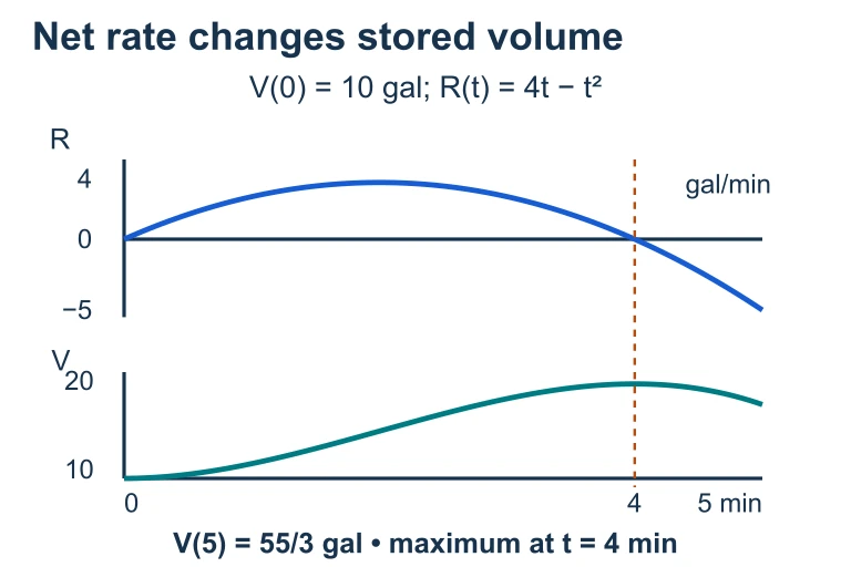For net flow R(t) = 4t − t² gal/min and 10 gal initially, V(t) = 10 + 2t² − t³/3. Volume peaks at t = 4 minutes, when the net rate changes from positive to negative.

SECTION 4

Mathematical Framework

FTC Part 1 — The Derivative of an Accumulation Function

FTC PART 1

d/dx [ ∫ₐˣ f(t) dt ] = f(x)

where f is continuous on [a, b] and a ≤ x ≤ b. The variable t is a dummy variable of integration; the result is a function of x alone.

FTC Part 1 states that if you define F(x) = ∫ from a to x of f(t) dt, then F is an antiderivative of f. The proof sketch proceeds by the definition of the derivative: F′(x) = lim as h→0 of [F(x + h) − F(x)]/h = lim as h→0 of [1/h · ∫ from x to x+h of f(t) dt]. Since f is continuous, the Mean Value Theorem for Integrals guarantees that the integral equals h · f(c) for some c between x and x + h. As h→0, c→x, and by continuity f(c)→f(x), giving F′(x) = f(x). This elegant argument transforms an integral into a derivative in a single step.

⚠

Chain Rule Extension

When the upper limit is a function g(x) instead of simply x, apply the chain rule: d/dx [ ∫ from a to g(x) of f(t) dt ] = f(g(x)) · g′(x). This extension appears frequently on the AP exam. For example, if F(x) = ∫ from 1 to x² of sin(t) dt, then F′(x) = sin(x²) · 2x.

FTC Part 2 — The Evaluation Theorem

FTC PART 2 (EVALUATION THEOREM)

∫ₐᵇ f(x) dx = F(b) − F(a)

where F is any antiderivative of f (i.e., F′(x) = f(x)) and f is continuous on [a, b]. The notation F(x) |ₐᵇ is shorthand for F(b) − F(a).

FTC Part 2 is the workhorse evaluation tool: it says that computing a definite integral requires only finding an antiderivative and evaluating at the endpoints. Without this theorem, every definite integral would need to be computed as a limit of Riemann sums — a far more laborious process. Note that the choice of antiderivative does not matter; if G(x) = F(x) + C, then G(b) − G(a) = [F(b) + C] − [F(a) + C] = F(b) − F(a). The constant of integration cancels.

ACCUMULATION FUNCTION DEFINITION

F(x) = ∫ₐˣ f(t) dt = net signed area from a to x

F(a) = 0 always (the integral from a to a is zero). F is increasing where f > 0, decreasing where f < 0, and has critical points where f = 0.

SECTION 5

Analyzing Accumulation Functions from Graphs

A signature AP Calculus AB question type provides the graph of f and asks you to analyze the accumulation function F(x) = ∫ from a to x of f(t) dt without ever writing an explicit formula. Because F′(x) = f(x), every feature of F can be deduced from the graph of f. Mastering this skill requires translating between the language of the integrand (height, sign, zero crossings) and the language of the accumulation function (slope, increasing/decreasing, extrema, concavity).

The green shaded region shows where f > 0 and F is increasing; the red shaded region shows where f < 0 and F is decreasing. The yellow dots at c₁ and c₂ mark zeros of f, corresponding to extrema of F. The annotations summarize the complete translation dictionary between f and F.

Feature of f(t)	Corresponding Feature of F(x)	Reasoning
f(x) > 0	F is increasing at x	F′(x) = f(x) > 0
f(x) < 0	F is decreasing at x	F′(x) = f(x) < 0
f(x) = 0 (sign change + to −)	F has a local maximum	F′ changes from positive to negative
f(x) = 0 (sign change − to +)	F has a local minimum	F′ changes from negative to positive
f is increasing	F is concave up	F″(x) = f′(x) > 0
f is decreasing	F is concave down	F″(x) = f′(x) < 0
f has a local extremum	F has an inflection point	F″ = f′ changes sign

Complete translation table between f and its accumulation function F

This translation table is your most powerful tool on the AP exam. When given a graph of f and asked about F, systematically identify the zeros of f (these become critical points of F), the sign of f on each interval (this determines where F increases or decreases), and whether f is increasing or decreasing on each subinterval (this determines the concavity of F). Always remember that F(a) = 0, which anchors your sketch of F at the starting point.

SECTION 6

Worked Example

Let us work through a multi-part problem that demonstrates both parts of the FTC, including the chain rule extension. This type of problem appears regularly on AP Calculus AB free-response sections.

Evaluating and Differentiating Accumulation Functions

1
Step 1 — State the Problem

Let g(x) = ∫ from 0 to x of (3t² − 12) dt. (a) Find g(3). (b) Find g′(x). (c) Find the x-values where g has a local minimum on the interval (−3, 3). (d) If h(x) = ∫ from 0 to x³ of (3t² − 12) dt, find h′(1).
2
Step 2 — Compute g(3) using FTC Part 2

Find an antiderivative of f(t) = 3t² − 12: F(t) = t³ − 12t. Apply the Evaluation Theorem: g(3) = F(3) − F(0) = (27 − 36) − (0 − 0) = −9.

g(3) = −9
3
Step 3 — Find g′(x) using FTC Part 1

By FTC Part 1, since f(t) = 3t² − 12 is continuous everywhere, g′(x) = f(x) = 3x² − 12. No chain rule is needed because the upper limit is simply x.

g′(x) = 3x² − 12
4
Step 4 — Find local minima of g

Set g′(x) = 0: 3x² − 12 = 0 → x² = 4 → x = ±2. Both lie in (−3, 3). Now apply the first derivative test. For x < −2, g′(x) = 3(−3)² − 12 = 15 > 0 (increasing). For −2 < x < 2, g′(0) = −12 < 0 (decreasing). For x > 2, g′(3) = 15 > 0 (increasing). At x = −2, g′ changes from positive to negative → local maximum. At x = 2, g′ changes from negative to positive → local minimum.

g has a local minimum at x = 2
5
Step 5 — Apply the Chain Rule Extension for h′(1)

Since h(x) = ∫ from 0 to x³ of (3t² − 12) dt, the upper limit is u = x³. By the chain rule extension: h′(x) = f(x³) · (d/dx)(x³) = (3(x³)² − 12) · 3x² = (3x⁶ − 12) · 3x². Evaluate at x = 1: h′(1) = (3 − 12) · 3 = (−9)(3) = −27.

h′(1) = −27

⚠

Common Exam Pitfall

Students often forget to multiply by the derivative of the upper limit when applying the chain rule extension. If the upper limit is anything other than x itself — such as x², sin(x), or 3x — you must include that extra factor. Similarly, if the lower limit is a function of x, the chain rule applies with a negative sign: d/dx [∫ from g(x) to b of f(t) dt] = −f(g(x)) · g′(x).

SECTION 7

Strengths, Limitations & Common Misconceptions

Strength / Use Case	Limitation / Pitfall
Converts definite integrals into simple antiderivative evaluations, eliminating the need for Riemann sums	Requires finding an antiderivative — not all functions have elementary antiderivatives (e.g., $e^{−x²}$ )
Accumulation functions allow analysis of F without ever finding an explicit formula for F	Students often confuse the graph of f with the graph of F; remember f is the derivative, not the function itself
The chain rule extension handles variable upper/lower limits seamlessly	Forgetting to multiply by the derivative of the upper (or lower) limit is the most common error
FTC Part 1 guarantees that every continuous function has an antiderivative	The continuity hypothesis is essential — discontinuities in f can invalidate the theorem
Provides a conceptual bridge between total change and rate of change	Definite integrals give net (signed) area, not total area; students forget to use absolute value for total distance

Strengths and common pitfalls of the Fundamental Theorem of Calculus

✦

KEY TAKEAWAY

The FTC is like knowing that a speedometer and an odometer are connected: if you know the speed at every moment (the integrand f), you can recover the total distance traveled (the integral). Conversely, if you track how total distance changes, the rate of that change gives you the speed. The most common errors on the AP exam arise from mixing up which function is which — always ask yourself: 'Is this function the rate or the accumulated total?'

SECTION 8

Connection to Advanced Theory

The Fundamental Theorem of Calculus as presented in AP Calculus AB is just the beginning of a rich family of results that generalize to higher dimensions and more abstract settings. Understanding where the FTC sits in this broader landscape provides motivation for future coursework and reveals the deep structural role the theorem plays in mathematics, physics, and engineering.

AP Calculus AB (FTC)	Advanced Generalization
∫ from a to b of f′(x) dx = f(b) − f(a)	Green's, Stokes', and the Divergence Theorems generalize this to line, surface, and volume integrals in multivariable calculus.
f must be continuous on [a, b]	Lebesgue's version relaxes this to almost-everywhere differentiability, allowing integration of far more pathological functions.
Accumulation function F(x) = ∫ from a to x of f(t) dt	In differential equations, integral equations define unknown functions via their accumulated effects — the FTC is the simplest case.
Applications to position, velocity, and acceleration	In physics, the FTC underpins the work-energy theorem, impulse-momentum theorem, and the relationship between electric field and potential.

How the FTC extends into advanced mathematics and science

If you continue to AP Calculus BC, you will encounter improper integrals (where the interval is infinite or the integrand is unbounded), which test the limits of the FTC. In multivariable calculus and beyond, theorems by Green, Stokes, and Gauss extend the same fundamental idea — that integrating a derivative over a region equals evaluating the original function on the boundary — to two and three dimensions. The core intuition you build here, that the total change equals the integral of the rate of change, remains valid and central in every one of these generalizations.

SECTION 9

Practice Problems

Question 1: CONCEPTUAL

Let F(x) = ∫ from 2 to x of f(t) dt, where f is continuous. If f(5) = 0 and f changes sign from positive to negative at t = 5, which statement about F is true?

A. F has a local minimum at x = 5
B. F has a local maximum at x = 5
C. F has an inflection point at x = 5
D. F(5) = 0
E. F is not differentiable at x = 5

Show answer (B)

By FTC Part 1, F′(x) = f(x). Since f(5) = 0, F′(5) = 0, so x = 5 is a critical point. Because f changes from positive to negative at t = 5, F′ changes from positive to negative, which by the First Derivative Test means F has a local maximum at x = 5. (A) is wrong because a local minimum requires a sign change from negative to positive. (C) is wrong because an inflection point of F requires f′ to change sign, which would mean f has an extremum — here f simply crosses zero. (D) is wrong because F(5) = ∫ from 2 to 5 of f(t) dt, which represents accumulated area and need not be zero. (E) is wrong because f is continuous, so FTC Part 1 guarantees F is differentiable.

Question 2: BASIC CALCULATION

Using the Fundamental Theorem of Calculus, evaluate ∫ from 1 to 4 of (6√t − 2/t²) dt.

A. 25/2
B. 57/4
C. 53/2
D. 28
E. 31/2

Show answer (C)

Rewrite the integrand: 6√t =

6t^{1/2}

and 2/t² =

2t^{−2}

. Find antiderivatives: ∫

6t^{1/2}

dt = 6 · (2/3)

t^{3/2}

4t^{3/2}

, and ∫

2t^{−2}

dt = 2 · (−1)

t^{−1}

= −2/t. So the antiderivative is F(t) =

4t^{3/2}

+ 2/t. Evaluate: F(4) − F(1) = [4(8) + 2/4] − [4(1) + 2/1] = [32 + 1/2] − [4 + 2] = 32.5 − 6 = 26.5 = 53/2. (A) 25/2 = 12.5 likely results from an antiderivative error. (B) 57/4 = 14.25 does not correspond to correct evaluation. (D) 28 likely omits the 2/t term. (E) 31/2 = 15.5 results from an error in evaluating at the lower bound.

Question 3: INTERMEDIATE

Let g(x) = ∫ from 1 to sin(x) of (t³ + 1) dt. Find g′(π/6).

A. 9√3 / 16
B. 9/8
C. √3 / 2
D. 9√3 / 8
E. 5√3 / 8

Show answer (A)

By the chain rule extension of FTC Part 1: g′(x) = f(sin(x)) · cos(x) where f(t) = t³ + 1. So g′(x) = (sin³(x) + 1) · cos(x). At x = π/6: sin(π/6) = 1/2, cos(π/6) = √3/2. Thus g′(π/6) = ((1/2)³ + 1) · (√3/2) = (1/8 + 1) · (√3/2) = (9/8)(√3/2) = 9√3/16. (B) 9/8 omits the cos(x) factor — a classic chain rule error. (C) √3/2 only accounts for cos(π/6) without evaluating the integrand. (D) 9√3/8 doubles the correct answer, likely from miscomputing 9/8 × √3/2. (E) 5√3/8 results from an arithmetic error in cubing 1/2.

Question 4: APPLIED

5 pts

A particle moves along the x-axis with velocity v(t) = t² − 4t + 3 for 0 ≤ t ≤ 5, where v is in meters per second and t is in seconds. The particle's position at t = 0 is x(0) = 2 meters. (a) Find the position function x(t). (b) At what time(s) does the particle change direction? Justify your answer. (c) Find the total distance traveled by the particle over [0, 5]. (d) Find the particle's average velocity over [0, 5].

Show answer

Rubric (5 points): (a) [1 point] By FTC Part 2, x(t) = x(0) + ∫ from 0 to t of v(s) ds = 2 + ∫ from 0 to t of (s² − 4s + 3) ds = 2 + [s³/3 − 2s² + 3s] from 0 to t = t³/3 − 2t² + 3t + 2. Award 1 point for the correct antiderivative with initial condition. (b) [1 point] The particle changes direction where v(t) = 0 and v changes sign. v(t) = t² − 4t + 3 = (t − 1)(t − 3) = 0 at t = 1 and t = 3. Sign analysis: v > 0 on (0, 1), v < 0 on (1, 3), v > 0 on (3, 5). Since v changes sign at both t = 1 and t = 3, the particle changes direction at t = 1 and t = 3. Award 1 point for correct times with sign-change justification. (c) [2 points] Total distance = ∫ from 0 to 5 of |v(t)| dt = ∫ from 0 to 1 of (t² − 4t + 3) dt + ∫ from 1 to 3 of −(t² − 4t + 3) dt + ∫ from 3 to 5 of (t² − 4t + 3) dt. First integral: [t³/3 − 2t² + 3t] from 0 to 1 = 1/3 − 2 + 3 = 4/3. Second integral: −[t³/3 − 2t² + 3t] from 1 to 3 = −[(9 − 18 + 9) − (1/3 − 2 + 3)] = −[0 − 4/3] = 4/3. Third integral: [t³/3 − 2t² + 3t] from 3 to 5 = (125/3 − 50 + 15) − (0) = 125/3 − 35 = 20/3. Total = 4/3 + 4/3 + 20/3 = 28/3 meters. Award 1 point for correct setup with absolute values and split intervals, 1 point for correct evaluation. (d) [1 point] Average velocity = (1/(5 − 0)) · ∫ from 0 to 5 of v(t) dt = (1/5)[x(5) − x(0)] = (1/5)[(125/3 − 50 + 15 + 2) − 2] = (1/5)(125/3 − 35) = (1/5)(20/3) = 4/3 m/s. Award 1 point for correct average velocity formula and evaluation.

Question 5: CRITICAL THINKING

3 pts

Let F(x) = ∫ from 0 to x of f(t) dt, where f is a continuous function on [−2, 6]. The following values are known: F(−1) = −3, F(0) = 0, F(2) = 5, F(4) = 5, F(6) = 1. (a) On which interval(s) must f have a zero? Justify using a theorem. (b) Does F have a critical point on (2, 6)? Justify. (c) Is it possible that f(x) > 0 for all x in [0, 2] and f(x) < 0 for all x in [4, 6]? Explain using the given data.

Show answer

Rubric (3 points): (a) [1 point] Since F′(x) = f(x), the values of F tell us about the integral of f. Note that F(2) − F(0) = 5 > 0, and F(6) − F(4) = 1 − 5 = −4 < 0. By the Mean Value Theorem applied to F on [0, 2], there exists c₁ in (0, 2) with F′(c₁) = f(c₁) = (5 − 0)/2 = 5/2 > 0. On [4, 6], there exists c₂ with F′(c₂) = f(c₂) = (1 − 5)/2 = −2 < 0. Since f is continuous and takes a positive value and a negative value, by the Intermediate Value Theorem, f must have a zero somewhere in (c₁, c₂) ⊂ (0, 6). More precisely, since F(2) = F(4) = 5, by the Mean Value Theorem on [2, 4], there exists c in (2, 4) with F′(c) = f(c) = 0. Award 1 point for correct application of MVT or IVT with justification. (b) [1 point] Yes. Since F(2) = 5 and F(4) = 5, by the Mean Value Theorem there exists some c in (2, 4) ⊂ (2, 6) where F′(c) = (F(4) − F(2))/(4 − 2) = 0. Since F′(c) = f(c) = 0, this c is a critical point of F. Award 1 point for correct identification and MVT justification. (c) [1 point] Yes, this is consistent. If f > 0 on [0, 2], then F is increasing on [0, 2], which matches F(0) = 0 < F(2) = 5. If f < 0 on [4, 6], then F is decreasing on [4, 6], which matches F(4) = 5 > F(6) = 1. These conditions are mutually compatible with the given data and with f being continuous (f would need to transition from positive to negative somewhere on (2, 4), which is allowed). Award 1 point for a correct and complete explanation.

SUMMARY

Summary

The Fundamental Theorem of Calculus establishes that differentiation and integration are inverse operations, unifying the two central ideas of calculus. FTC Part 1 states that if F(x) = ∫ from a to x of f(t) dt and f is continuous, then F′(x) = f(x) — the derivative of an accumulation function recovers the original integrand. FTC Part 2 (the Evaluation Theorem) states that ∫ from a to b of f(x) dx = F(b) − F(a), converting definite integrals into simple endpoint evaluations of any antiderivative.

When analyzing accumulation functions, remember the translation table: where f > 0, F increases; where f < 0, F decreases; zeros of f correspond to critical points of F; and extrema of f correspond to inflection points of F. The chain rule extension — d/dx [∫ from a to g(x) of f(t) dt] = f(g(x)) · g′(x) — is essential for problems with non-trivial upper limits. These tools appear throughout both the multiple-choice and free-response sections of the AP Calculus AB exam and form the foundation for all subsequent integration techniques.