Exponential Models with Differential Equations - AP Calculus AB

SECTION 1

Historical Context & Motivation

The idea that a quantity's rate of change is proportional to the quantity itself is one of the most powerful and enduring relationships in mathematics. Long before the formal language of calculus existed, scholars noticed that populations, compound interest, and radioactive substances all seemed to follow a common pattern: the bigger something gets, the faster it grows — or conversely, the less there is of something, the slower it decays. This observation eventually crystallized into the exponential differential equation dy/dt = ky, a deceptively simple equation whose solution, y = Ce^kt, appears in virtually every branch of science and engineering.

1683 • Jacob Bernoulli & Compound Interest

While studying the problem of continuously compounded interest, Jacob Bernoulli discovered the limiting value (1 + 1/n)ⁿ as n → ∞, which converges to the constant e ≈ 2.71828.

1798 • Malthus & Population Growth

Thomas Malthus published "An Essay on the Principle of Population," arguing that unchecked populations grow geometrically — an observation that maps directly onto the exponential growth model dP/dt = kP.

1896 • Becquerel & Radioactive Decay

Henri Becquerel's discovery of radioactivity opened a new domain for exponential decay. Ernest Rutherford later formalized the half-life concept, showing that radioactive substances obey dN/dt = −λN.

1928 • Newton's Law of Cooling Formalized

Although Newton proposed his cooling law in 1701, its rigorous treatment using differential equations matured in the early twentieth century, linking temperature change dT/dt = −k(T − Tₛ) to exponential decay toward ambient temperature.

The central question these developments converge upon is this: given only the knowledge that a rate of change is proportional to a current value, can we predict the future behavior of the system exactly? The answer is a resounding yes, and the tool that unlocks this prediction is separation of variables — the technique that transforms the differential equation dy/dt = ky into the explicit solution y = Ce^kt. Understanding this equation and its variations is essential for the AP Calculus AB exam.

SECTION 2

Core Principles & Definitions

Before diving into solution techniques, it is essential to anchor the foundational ideas that make exponential models work. Every exponential model rests on a single structural assumption: the instantaneous rate of change of a quantity is directly proportional to the current value of that quantity. From this single assumption, a remarkably rich family of solutions emerges.

The Differential Equation dy/dt = ky

This is the defining equation. The constant k is the relative growth rate. When k > 0 the quantity grows exponentially; when k < 0 it decays exponentially.

The General Solution y = Ceᵏᵗ

Solving by separation of variables yields y = Ce^kt, where C = y(0) is the initial condition. This is the only function family satisfying the equation.

Exponential Growth (k > 0)

When the proportionality constant is positive, the solution curves sweep upward without bound. Population models and continuously compounded interest exhibit this behavior. The doubling time is t₂ = ln 2 / k.

Exponential Decay (k < 0)

A negative proportionality constant drives the quantity toward zero asymptotically. Radioactive decay and cooling processes follow this pattern. The half-life is t₁/₂ = ln 2 / |k|.

Initial Value Problems (IVPs)

On the AP exam, you are typically given dy/dt = ky together with a specific value y(t₀) = y₀. The initial condition pins down C, converting the general solution into a unique particular solution.

✦

KEY TAKEAWAY

Think of exponential growth like a snowball rolling downhill: the bigger the snowball gets, the more surface area it has to pick up snow, so it grows faster and faster. Exponential decay is the reverse — imagine an ice cube melting in warm air. The smaller it gets, the less surface area is exposed, so the melting rate slows proportionally. In both cases, the rate of change scales with the current size, which is precisely what dy/dt = ky encodes.

SECTION 3

Visualizing Exponential Growth & Decay

A graph is worth more than a page of algebra when it comes to internalizing the behavior of exponential functions. The diagram below plots several solution curves of dy/dt = ky for both positive and negative values of k, all sharing the same initial condition y(0) = 4. Observe how the sign and magnitude of k dictate whether the curve climbs steeply, climbs gently, or decays toward zero.

All four curves share the initial value y(0) = 4 (green dot). The pink curve (k = 0.5) and violet curve (k = 0.25) show exponential growth — larger k means steeper ascent. The cyan curve (k = −0.25) and amber curve (k = −0.5) show exponential decay — the quantity approaches zero but never reaches it.

Several features stand out in this diagram. First, every curve passes through the point (0, 4) because C = y(0) = 4 for all four. Second, the growth curves are concave up: as y increases, dy/dt = ky also increases, accelerating the climb. Third, the decay curves are concave up as well (since the second derivative y″ = k²y > 0), but they are decreasing. The horizontal axis y = 0 acts as a horizontal asymptote for every decay curve — the quantity never actually reaches zero, a fact with deep physical implications in contexts like radioactive decay.

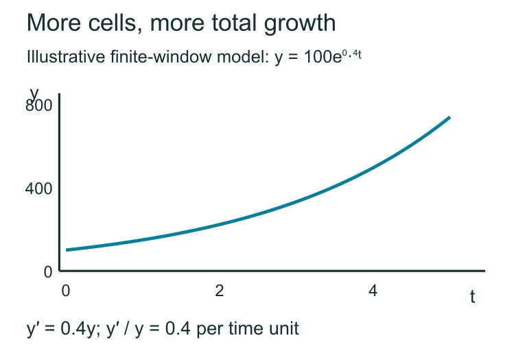A researcher looks through a microscope beside a closed culture vessel,sample containers and an illustrative cell inset. In the model y = 100e^(0.4t), the relative growth rate stays at 0.4 while total growth y′ = 0.4y increases with the population.

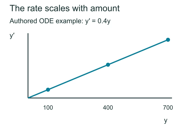In the model y = 100e^(0.4t), the relative growth rate stays at 0.4 while total growth y′ = 0.4y increases with the population.

SECTION 4

Mathematical Framework — Derivation & Formulas

The derivation of the exponential model from its differential equation is a textbook application of separation of variables. We begin with dy/dt = ky, separate the variables so that all y-terms appear on one side and all t-terms on the other, integrate both sides, and solve for y explicitly. This process is a cornerstone of the AP Calculus AB curriculum and appears regularly on both the multiple-choice and free-response sections.

DIFFERENTIAL EQUATION

dy/dt = ky

y = y(t) is the quantity as a function of time, k is the constant of proportionality (growth rate if k > 0, decay rate if k < 0), and t is the independent variable (usually time).

SEPARATION OF VARIABLES

(1/y) dy = k dt → ∫(1/y) dy = ∫k dt → ln|y| = kt + C₁

We divide both sides by y (assuming y ≠ 0), multiply both sides by dt, and integrate. The antiderivative of 1/y is ln|y|, and the antiderivative of k is kt. The arbitrary constant C₁ absorbs both constants of integration.

EXPONENTIATION

|y| = e^(kt + C₁) = e^(C₁) × e^(kt) → y = Ce^(kt) where C = ±e^(C₁)

Exponentiating both sides removes the natural log. The constant C = ±e^C₁ is determined by the initial condition. If y(0) = y₀, then C = y₀.

GENERAL SOLUTION (IVP FORM)

y(t) = y₀ × e^(kt)

y₀ is the initial value y(0). This formula completely determines y for all t once y₀ and k are known. For growth, k > 0. For decay, k < 0.

⚠

AP Exam Tip

On the AP Calculus AB exam, you are expected to derive y = Ce^kt from dy/dt = ky by separation of variables. Simply writing the solution without showing the separation and integration steps will not earn full credit on free-response questions. Always show the separation, the integrals, the exponentiation, and the application of the initial condition.

SECTION 5

Detailed Breakdown — Growth, Decay & Special Formulas

While the general solution y = y₀e^kt covers all cases, real-world problems often present information indirectly. You might be given a half-life, a doubling time, a percentage rate, or two data points and asked to find k. The diagram below provides a decision flowchart for identifying which sub-formula to use, and the table that follows catalogs the most common variations.

This flowchart guides you from recognizing a differential equation of the form dy/dt = ky through determining whether the model represents growth or decay, and finally to the relevant time-constant formula. The orange box on the right summarizes how to determine k when you are given data points or a half-life.

Scenario	Given Information	Formula for k	Solution
Doubling time t₂	y doubles every t₂ units	k = ln 2 / t₂	y = y₀ × 2^t/t₂
Half-life t₁/₂	y halves every t₁/₂ units	k = −ln 2 / t₁/₂	y = y₀ × (1/2)^t/t₁/₂
Two data points	y(t₁) = y₁ and y(0) = y₀	k = ln(y₁ / y₀) / t₁	y = y₀ × e^kt
Percentage rate r	y grows at r% per unit time	k = ln(1 + r/100)	y = y₀ × e^kt

Common exponential model scenarios and how to determine k

SECTION 6

Worked Example — Radioactive Decay

Let us work through a complete example of the type you would encounter on the AP Calculus AB free-response section. This problem requires setting up the differential equation, solving it by separation of variables, determining the constant k from a half-life, and then using the model to answer a prediction question.

ℹ

Problem Statement

A radioactive substance has a half-life of 8 years. At time t = 0, a sample contains 200 grams. The rate of decay is proportional to the amount present. (a) Write a differential equation for the amount A(t). (b) Solve the differential equation. (c) Find the value of k. (d) How much substance remains after 20 years?

Full Solution

1
Step 1 — Write the Differential Equation

Since the rate of decay is proportional to the amount present, we write dA/dt = kA, where k is a negative constant (because the substance is decaying). The initial condition is A(0) = 200.

dA/dt = kA, A(0) = 200
2
Step 2 — Separate Variables and Integrate

Divide both sides by A and multiply by dt: (1/A) dA = k dt. Integrate both sides: ∫(1/A) dA = ∫k dt, which yields ln|A| = kt + C₁. Exponentiate: A = Ce^kt, where C = ±e^C₁.

A(t) = Ceᵏᵗ
3
Step 3 — Apply the Initial Condition

Substituting t = 0: A(0) = Ce⁰ = C = 200. Therefore the particular solution is A(t) = 200e^kt.

A(t) = 200eᵏᵗ
4
Step 4 — Determine k from the Half-Life

The half-life is 8 years, so A(8) = 100. Substituting: 100 = 200e^8k. Dividing by 200: 1/2 = e^8k. Taking ln of both sides: ln(1/2) = 8k, so k = −ln 2 / 8 ≈ −0.08664.

k = −ln 2 / 8 ≈ −0.08664
5
Step 5 — Find A(20)

Substituting t = 20: A(20) = 200e^{(−ln 2 / 8)(20)} = 200e^{−2.5 ln 2} = 200 × 2^−2.5 = 200 / (2^2.5) = 200 / (4√2) ≈ 200 / 5.6569 ≈ 35.36 grams.

A(20) ≈ 35.36 grams

SECTION 7

Strengths & Limitations of the Exponential Model

The exponential model is elegant and widely applicable, but it carries inherent limitations that you should understand both for the AP exam and for scientific literacy. Recognizing when this model is appropriate — and when it breaks down — is a higher-order skill that distinguishes strong exam responses from merely procedural ones.

Strengths	Limitations
Analytically solvable — the closed-form solution y = y₀eᵏᵗ allows exact predictions without numerical methods.	Assumes unlimited resources — real populations face carrying capacity constraints, making the model unrealistic for long-term biological forecasting.
Universal applicability — the same mathematical structure describes phenomena across physics, biology, chemistry, finance, and pharmacology.	Constant relative rate — the model requires k to be truly constant. In reality, rates often change due to temperature, competition, or policy shifts.
Easily parameterized — only two quantities (y₀ and k) fully determine the model, making it ideal for situations with limited data.	Growth without bound — for k > 0, the model predicts y → ∞, which is physically impossible in all real-world systems.
Excellent short-term approximation — even when the true model is logistic or more complex, exponential behavior dominates early dynamics.	Cannot model oscillations, thresholds, or saturation without modification. Phenomena with feedback loops require differential equations beyond dy/dt = ky.

Comparative analysis of the exponential model

✦

KEY TAKEAWAY

Think of the exponential model as a first-order approximation, much like a tangent line is a linear approximation to a curve. It captures the essential behavior near the initial conditions beautifully, but the further you extrapolate, the more reality diverges. In AP Calculus AB, when a problem says "the rate is proportional to the amount," you are being told to use this model. In AP Calculus BC and beyond, the logistic model dy/dt = ky(1 − y/L) addresses the limitation of unbounded growth.

SECTION 8

Connection to Advanced Theory

The exponential differential equation dy/dt = ky is the simplest member of a family of autonomous first-order ordinary differential equations. Understanding it well prepares you not only for the AP Calculus AB exam but also for the richer models you will encounter in BC Calculus, differential equations courses, and applied mathematics. The table below contrasts the pure exponential model with several extensions, each of which addresses one of the limitations discussed in Section 7.

Feature	Exponential Model (AB)	Logistic Model (BC & Beyond)
Differential Equation	dy/dt = ky	dy/dt = ky(1 − y/L)
Solution	y = y₀eᵏᵗ	y = L / (1 + Ae⁻ᵏᵗ)
Long-term behavior (k > 0)	y → ∞ (unbounded)	y → L (carrying capacity)
Inflection point	No inflection (always concave up)	At y = L/2 (fastest growth)
AP Exam Coverage	Tested on AB and BC	Tested on BC only
Solution method	Separation of variables	Partial fractions + separation

Exponential vs. Logistic: from AB to BC

Even within the AB curriculum, recognizing the exponential model's place in the broader landscape deepens your conceptual understanding. When a free-response question asks you to comment on whether a model is reasonable for large t, the answer often involves acknowledging that real-world growth cannot continue exponentially forever. This kind of critical analysis earns communication points on the exam. Additionally, Newton's Law of Cooling — dT/dt = −k(T − Tₛ) — is an extension where the difference (T − Tₛ) plays the role of y, and the equilibrium temperature Tₛ acts as a horizontal asymptote, a concept that bridges the pure exponential model to more nuanced applications.

A steaming coffee cup and a cool liquid cup with condensation, each probed, with a shared room-reference probe between them. With ambient temperature 22 °C and k > 0, T′ = −k(T − 22). A warmer liquid cools and a cooler liquid warms, both approaching ambient temperature.

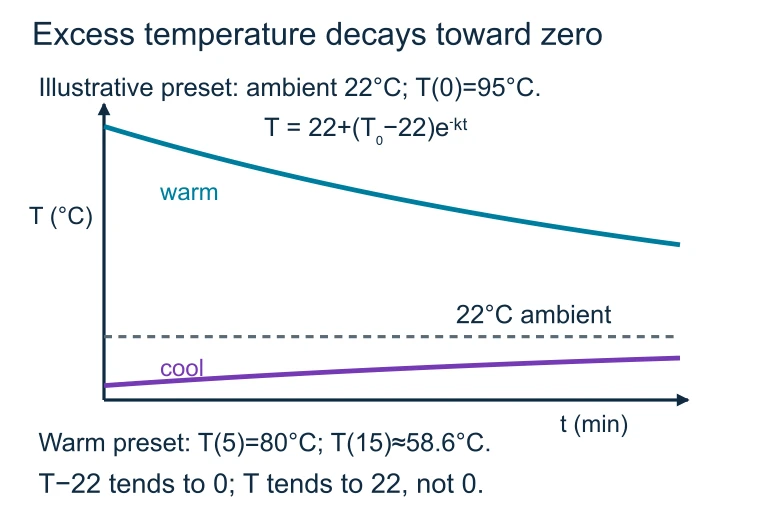With ambient temperature 22 °C and k > 0, T′ = −k(T − 22). A warmer liquid cools and a cooler liquid warms, both approaching ambient temperature.

SECTION 9

Practice Problems

Question 1: CONCEPTUAL

A population P satisfies the differential equation dP/dt = 0.03P with P(0) = 500. Which of the following statements best describes the behavior of P(t) as t increases?

A. P(t) increases at a constant rate of 0.03 units per year.
B. P(t) increases and the rate of increase itself increases over time.
C. P(t) increases toward a horizontal asymptote.
D. P(t) decreases exponentially toward zero.
E. P(t) increases linearly with slope 15.

Show answer (B)

The correct answer is B. Since k = 0.03 > 0, the solution is P(t) = 500e^0.03t, which is an increasing exponential function. Moreover, dP/dt = 0.03P increases as P increases, so the rate of increase accelerates. Choice A is wrong because dP/dt = 0.03P is not constant — it depends on P. Choice C describes logistic behavior (bounded growth), not pure exponential growth. Choice D is wrong because k > 0 means growth, not decay. Choice E is wrong because the initial rate is 0.03 × 500 = 15, but the rate does not remain constant; it grows with P.

Question 2: BASIC CALCULATION

A substance decays according to dA/dt = −0.05A with A(0) = 80 grams. What is the amount remaining after 10 units of time?

A. 80e^0.5 ≈ 131.88 grams
B. 80e^−0.5 ≈ 48.52 grams
C. 80 − 0.05(10) = 79.5 grams
D. 80e⁻⁵ ≈ 0.54 grams
E. 40 grams

Show answer (B)

The correct answer is B. Solving dA/dt = −0.05A with A(0) = 80 gives A(t) = 80e^−0.05t. At t = 10: A(10) = 80e^−0.5 ≈ 48.52 grams. Choice A incorrectly uses a positive exponent, yielding growth instead of decay. Choice C treats the decay as linear (subtracting the rate times time), ignoring that this is exponential. Choice D uses an exponent of −5 instead of −0.5, likely confusing k × t = 0.05 × 10 = 0.5 with 5. Choice E assumes t = 10 is exactly the half-life, but the half-life is ln 2 / 0.05 ≈ 13.86, not 10.

Question 3: INTERMEDIATE

A bacterial culture grows according to dy/dt = ky. At t = 0, there are 1,000 bacteria, and at t = 3 hours, there are 8,000 bacteria. What is the population at t = 5 hours?

A. 1000 × 8^5/3 ≈ 32,000
B. 40,000
C. 1000e⁵ ≈ 148,413
D. 13,333
E. 24,000

Show answer (A)

The correct answer is A. From y(0) = 1000 and y(3) = 8000: 8000 = 1000e^3k, so e^3k = 8, giving k = ln 8 / 3 = ln 2³ / 3 = ln 2. Then y(5) = 1000e^{5 ln 2} = 1000 × 2⁵ = 32,000. Equivalently, since the culture multiplies by 8 every 3 hours, y(5) = 1000 × 8^5/3 = 1000 × (2³)^5/3 = 1000 × 2⁵ = 32,000. Choice B (40,000) likely comes from a linear extrapolation error. Choice C uses k = 1 instead of k = ln 2. Choice D (13,333) results from treating the growth as linear: 1000 + (7000/3)(5). Choice E (24,000) might come from incorrectly multiplying 8000 × 3.

Question 4: APPLIED

3 pts

A pharmaceutical company models drug concentration C(t) (in mg/L) in a patient's bloodstream by the differential equation dC/dt = −kC. After an injection, C(0) = 12 mg/L and the drug's half-life in the body is 4 hours. (a) Find the value of k. (b) Write the particular solution for C(t). (c) Determine the concentration at t = 10 hours.

Show answer

Part (a) — 1 point: Using the half-life condition: C(4) = 6 = 12e^−4k → 1/2 = e^−4k → −4k = ln(1/2) = −ln 2 → k = ln 2 / 4 ≈ 0.1733. (1 point for correct k) Part (b) — 1 point: Separate variables: ∫(1/C) dC = ∫−k dt → ln|C| = −kt + A → C = C₀e^−kt. Using C(0) = 12: C(t) = 12e^{−(ln 2 / 4)t}, or equivalently C(t) = 12 · (1/2)^t/4. (1 point for correct particular solution) Part (c) — 1 point: C(10) = 12e^{−(ln 2 / 4)(10)} = 12e^{−2.5 ln 2} = 12 · 2^−2.5 = 12 / (4√2) = 3√2 / 2 ≈ 2.121 mg/L. (1 point for correct computation)

Question 5: CRITICAL THINKING

3 pts

Let f be a twice-differentiable function satisfying df/dt = kf for some constant k ≠ 0. (a) Show that f″(t) = k²f(t) for all t. (b) Use part (a) to explain why the graph of f is always concave up when f(t) > 0, regardless of the sign of k. (c) Explain why this concavity result means that exponential decay curves never cross the t-axis.

Show answer

Part (a) — 1 point: Differentiating both sides of f′(t) = kf(t) with respect to t: f″(t) = kf′(t) = k(kf(t)) = k²f(t). Since this uses only the chain rule and the original DE, it holds for all t. (1 point for correct differentiation and substitution.) Part (b) — 1 point: Since k² > 0 for all k ≠ 0, we have f″(t) = k²f(t). When f(t) > 0, it follows that f″(t) = k²f(t) > 0, which means the graph is concave up. This holds whether k is positive (growth) or negative (decay), because k² is always positive. (1 point for connecting k² > 0 and f > 0 to concavity.) Part (c) — 1 point: For exponential decay with f(0) > 0, f is positive and decreasing. Since f is concave up whenever f > 0, the curve bends upward (toward the horizontal asymptote y = 0) rather than downward through it. A concave-up decreasing function that starts positive approaches the t-axis asymptotically but can never reach or cross zero. Formally, if f(t₀) = 0 at some finite t₀, then by the uniqueness theorem for ODEs, f would be the zero function — a contradiction with f(0) > 0. The concavity argument provides the geometric intuition for this analytical fact. (1 point for a clear geometric or analytical explanation.)

SUMMARY

Summary — Exponential Models with Differential Equations

Summary

The exponential differential equation dy/dt = ky states that the rate of change of a quantity is proportional to the quantity itself. Solving by separation of variables — separating, integrating, exponentiating, and applying the initial condition y(0) = y₀ — yields the unique particular solution y(t) = y₀e^kt. When k > 0, the model describes exponential growth with doubling time t₂ = ln 2 / k; when k < 0, it describes exponential decay with half-life t₁/₂ = ln 2 / |k|.

On the AP Calculus AB exam, always show your full derivation — separate variables, write both integrals, exponentiate, and apply the initial condition — to earn full credit on free-response questions. Remember that the constant k can be determined from a half-life, a doubling time, or a second data point using k = ln(y₁/y₀)/t₁. This model is the foundation for understanding more complex equations like the logistic model, Newton's Law of Cooling, and coupled systems you will encounter in advanced courses.