Exploring Accumulations of Change - AP Calculus AB

SECTION 1

Historical Context & Motivation

Long before the formal machinery of calculus existed, mathematicians grappled with a deceptively simple question: if you know how fast something is changing at every instant, can you recover the total amount of change that has occurred? Ancient Greek geometers confronted this challenge when they tried to compute areas bounded by curves—regions that refused to yield to the straightforward length-times-width formulas of rectangles. The insight that such areas could be approximated by summing many thin slices was the conceptual seed from which the entire theory of accumulation of change would grow. This idea—breaking a whole into infinitely many infinitesimal pieces and reassembling them—is the beating heart of integral calculus.

~250 BCE • Archimedes' Method of Exhaustion

Archimedes approximated the area of a parabolic segment by inscribing successively finer triangles, effectively summing slices to compute a curved area—an ancient precursor to integration.

1635 • Cavalieri's Principle of Indivisibles

Bonaventura Cavalieri formalized the idea that a region could be decomposed into infinitely many parallel line segments, enabling area computations through systematic summation.

1668 • Riemann-Sum Precursors by Wallis and Gregory

John Wallis and James Gregory developed algebraic techniques for summing series of powers, laying the arithmetic groundwork for what would become Riemann sums.

1687 • Newton and Leibniz Formalize Calculus

Isaac Newton and Gottfried Wilhelm Leibniz independently published frameworks linking rates of change (derivatives) to accumulated change (integrals), establishing the Fundamental Theorem of Calculus.

1854 • Riemann's Rigorous Definition

Bernhard Riemann gave the first precise definition of the definite integral as the limit of partition sums, providing the rigorous foundation that modern calculus courses still teach.

The central question that drove centuries of mathematical innovation remains the one you will master in this lesson: given a function that describes a rate of change, how do we determine the total accumulated quantity over an interval? Whether that rate represents velocity, population growth, or energy flow, the strategy is the same: partition the interval, approximate each piece, sum them up, and take the limit as the partitions grow infinitely fine.

SECTION 2

Core Principles & Definitions

At its foundation, the concept of accumulation of change rests on a small set of interconnected ideas that together explain why integration works and what it measures. Before diving into formulas and computation, it is essential to internalize these principles conceptually, because the AP Calculus AB exam frequently tests whether students understand why a definite integral yields a net accumulation, not just how to evaluate one.

Rate × Time ≈ Change

If a rate of change f(t) is approximately constant over a small interval Δt, then the change in the accumulated quantity is approximately f(t) · Δt. This is the fundamental building block of every Riemann sum.

Partition, Approximate, Sum, Limit

To find the total accumulation, we partition the interval [a, b] into n subintervals, approximate the change on each subinterval, sum the approximations, and take the limit as n → ∞. The result is the definite integral.

Net vs. Total Accumulation

The definite integral ∫ₐᵇ f(x) dx computes the net (signed) accumulation. When f is negative, the contribution subtracts from the total. Total accumulation uses ∫ₐᵇ |f(x)| dx to count all change as positive.

Units of the Integral

The units of ∫ₐᵇ f(x) dx are always (units of f) × (units of x). If f is in meters per second and x is in seconds, the integral has units of meters. This dimensional check is a powerful error-detection tool.

The Accumulation Function

The function F(x) = ∫ₐˣ f(t) dt defines a new function whose value at any x equals the net accumulation of f from a to x. Its derivative is F′(x) = f(x), which is the essence of the Fundamental Theorem of Calculus.

✦

KEY TAKEAWAY

Think of accumulation like a rain gauge. The rate of rainfall (inches per hour) varies throughout a storm. At any given moment the gauge isn't measuring the rate—it's collecting the total. Integration is the mathematical rain gauge: it takes a rate function and returns the total quantity that has accumulated. When the rate is high, the gauge fills faster; when the rate drops to zero or goes negative (evaporation), the total pauses or decreases. The definite integral simply formalizes this everyday observation into a precise mathematical operation.

SECTION 3

Visual Explanation — Riemann Sums & Area Under a Curve

The most powerful visual for understanding accumulation is the area-under-the-curve interpretation. When we graph a rate function f(x) on the vertical axis against the independent variable x on the horizontal axis, the signed area between the curve and the x-axis over an interval [a, b] equals the net accumulation. The diagram below illustrates this idea using a left Riemann sum with six subintervals approximating the definite integral of a sample function.

The six cyan rectangles represent the left Riemann sum approximation. Each rectangle's height equals the function value at the left endpoint of its subinterval, and its width equals Δx = 1. The violet curve shows the actual function f(x). As n increases and Δx shrinks toward zero, the total area of the rectangles converges to the exact value of the definite integral.

Notice that some rectangles overshoot the curve (overestimates) and others undershoot (underestimates). Whether a left Riemann sum overestimates or underestimates depends on whether the function is decreasing or increasing on each subinterval. On the AP exam, you will frequently be asked to determine whether a particular Riemann sum is an overestimate or underestimate given information about the function's monotonicity or concavity. The key insight is that refinement—increasing n—always drives the approximation closer to the true integral, and in the limit the error vanishes entirely.

SECTION 4

Mathematical Framework

The transition from Riemann sums to the definite integral is captured by a precise limiting process. In this section we formalize the notation and establish the key equations that govern accumulation of change. These formulas form the computational backbone of everything you will do with integrals on the AP Calculus AB exam.

RIEMANN SUM

Sₙ = Σᵢ₌₁ⁿ f(xᵢ*) · Δx

Here [a, b] is partitioned into n subintervals of equal width Δx = (b − a)/n. Each xᵢ* is a sample point in the i-th subinterval. Common choices: left endpoint (xᵢ* = a + (i−1)Δx), right endpoint (xᵢ* = a + iΔx), or midpoint.

DEFINITE INTEGRAL

∫ₐᵇ f(x) dx = lim(n→∞) Σᵢ₌₁ⁿ f(xᵢ*) · Δx

The definite integral is defined as the limit of Riemann sums as the number of subintervals approaches infinity (equivalently, as Δx → 0). If this limit exists and is the same regardless of the choice of sample points, then f is integrable on [a, b].

ACCUMULATION FUNCTION

F(x) = ∫ₐˣ f(t) dt

F(x) represents the net accumulation of f from the fixed lower limit a to the variable upper limit x. The variable t is a dummy variable of integration. By the Fundamental Theorem of Calculus (Part 1), F′(x) = f(x), so the derivative of the accumulation function returns the original rate function.

EVALUATION THEOREM (FTC PART 2)

∫ₐᵇ f(x) dx = F(b) − F(a)

If F is any antiderivative of f (meaning F′(x) = f(x) for all x in [a, b]), then the definite integral equals the net change in F over the interval. This theorem transforms the limit-of-sums definition into a practical computation: find an antiderivative, evaluate it at the endpoints, and subtract.

💡

AP Exam Tip

The AP exam often provides a table of values for a rate function and asks you to approximate the definite integral using a left, right, midpoint, or trapezoidal sum. Be sure you can set up these sums quickly. Also remember: if you are given f′(x) and asked for the change in f, you compute ∫ₐᵇ f′(x) dx = f(b) − f(a). The integral of a rate of change gives the net change in the original quantity.

A stirred transparent tank has one upper inlet and one lower outlet with a valve. The exact diagram links its 100 L salt balance to a computed approach to equilibrium. For net flow R(t) = 4t − t² gal/min and 10 gal initially, V(t) = 10 + 2t² − t³/3. Volume peaks at t = 4 minutes, when the net rate changes from positive to negative.

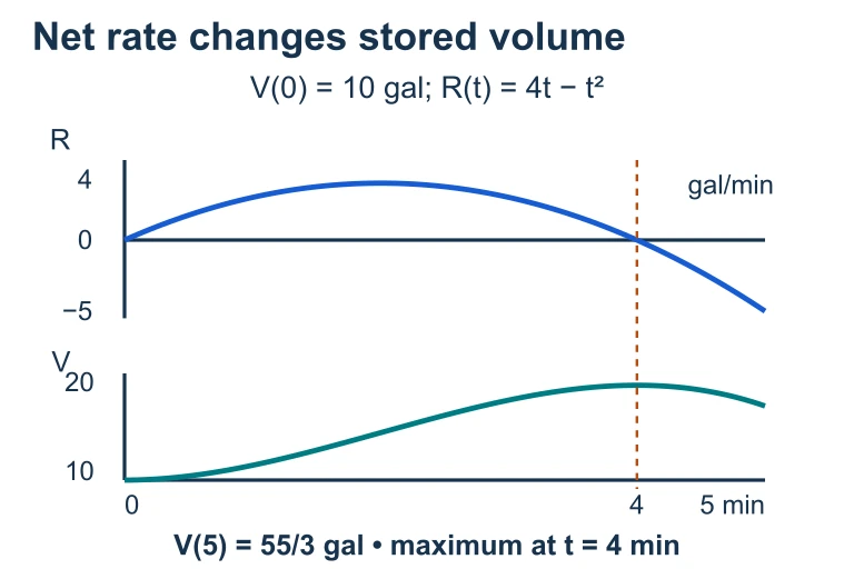For net flow R(t) = 4t − t² gal/min and 10 gal initially, V(t) = 10 + 2t² − t³/3. Volume peaks at t = 4 minutes, when the net rate changes from positive to negative.

SECTION 5

Approximation Methods & Their Properties

When an antiderivative is not available—either because the function is defined only by a table of data or because no closed-form antiderivative exists—we rely on numerical approximation techniques. On the AP Calculus AB exam, you are expected to know four primary methods: the left Riemann sum, the right Riemann sum, the midpoint Riemann sum, and the trapezoidal sum. Each method chooses a different representative height (or shape) for each subinterval, producing different levels of accuracy.

Four subintervals illustrate each approximation method applied to the same concave-down, increasing-then-decreasing curve (violet). The left Riemann sum uses left-endpoint heights, the right Riemann sum uses right-endpoint heights, the midpoint sum uses midpoint heights, and the trapezoidal sum connects left and right endpoints with a straight line, forming trapezoids.

Method	Formula for n Equal Subintervals	Error Behavior
Left Riemann	Δx · [f(x₀) + f(x₁) + … + f(xₙ₋₁)]	Under for increasing f; over for decreasing f
Right Riemann	Δx · [f(x₁) + f(x₂) + … + f(xₙ)]	Over for increasing f; under for decreasing f
Midpoint	Δx · [f(m₁) + f(m₂) + … + f(mₙ)], mᵢ = (xᵢ₋₁ + xᵢ)/2	Under for concave up; over for concave down
Trapezoidal	(Δx/2) · [f(x₀) + 2f(x₁) + 2f(x₂) + … + 2f(xₙ₋₁) + f(xₙ)]	Over for concave up; under for concave down

Summary of Riemann sum and trapezoidal approximation formulas

SECTION 6

Worked Example — Accumulation from a Table

A common AP Calculus AB scenario provides a table of rate-function values at discrete points and asks you to approximate the total accumulation. Let's work through a complete example that mirrors the style and rigor of the AP free-response section.

ℹ

Problem Statement

Water flows into a tank at a rate modeled by R(t) liters per minute. Selected values of R(t) are given in the table below. Using a right Riemann sum with four subintervals indicated by the table, approximate ∫₀⁸ R(t) dt and explain its meaning in context.

t (minutes)	0	2	3	5	8
R(t) (L/min)	4	7	9	6	3

Table of rate values for R(t)

Solution: Right Riemann Sum with Unequal Subintervals

1
Step 1 — Identify the Subintervals

The five data points create four subintervals: [0, 2], [2, 3], [3, 5], and [5, 8]. Notice that these subintervals have unequal widths: Δt₁ = 2, Δt₂ = 1, Δt₃ = 2, Δt₄ = 3. This is common on the AP exam—do not assume equal subintervals.
2
Step 2 — Determine the Right-Endpoint Values

For a right Riemann sum, the height of each rectangle is the function value at the right endpoint of that subinterval. These are: R(2) = 7, R(3) = 9, R(5) = 6, R(8) = 3.
3
Step 3 — Compute Each Product (Rate × Width)

Multiply each right-endpoint value by the corresponding subinterval width:

R(2)·Δt₁ = 7 × 2 = 14; R(3)·Δt₂ = 9 × 1 = 9; R(5)·Δt₃ = 6 × 2 = 12; R(8)·Δt₄ = 3 × 3 = 9
4
Step 4 — Sum the Products

Add the four contributions:

∫₀⁸ R(t) dt ≈ 14 + 9 + 12 + 9 = 44 liters
5
Step 5 — Interpret in Context

Since R(t) is in liters per minute and t is in minutes, the integral has units of liters. The approximation tells us that approximately 44 liters of water flow into the tank during the first 8 minutes. On the AP exam, failing to include the contextual interpretation—units and meaning—will cost you a rubric point.

SECTION 7

Strengths & Limitations of Approximation Methods

Not all approximation methods are created equal, and understanding their trade-offs helps you make strategic choices on the AP exam. The trapezoidal rule and midpoint rule are generally more accurate than left or right Riemann sums for the same number of subintervals, but each method has specific scenarios where it excels or falls short. This section compares the four primary methods along several dimensions that matter both computationally and conceptually.

Criterion	Left / Right Riemann	Midpoint	Trapezoidal
Accuracy (smooth f)	Error ∝ 1/n (first order)	Error ∝ 1/n² (second order)	Error ∝ 1/n² (second order)
Data requirements	Function values at endpoints only	Function values at midpoints	Function values at endpoints only
Over/under guarantee	Yes, if f is monotonic	Yes, if f has constant concavity	Yes, if f has constant concavity
Works with unequal subintervals?	Yes—multiply each f-value by its own Δx	Yes, but midpoints must be computable	Yes—apply trapezoid formula per subinterval
AP exam frequency	Very common (table-based FRQs)	Occasional (requires midpoint data)	Very common (table-based FRQs)

Comparison of integral approximation methods for AP Calculus AB

✦

KEY TAKEAWAY

Choosing an approximation method is like choosing a measuring tool. Left and right Riemann sums are like using a ruler with coarse markings—quick and easy, but not highly precise. The trapezoidal rule is like upgrading to a ruler with finer markings; it captures the slope between consecutive data points and thereby reduces the error. The midpoint rule is surprisingly powerful—like sampling at the optimal location within each interval—and often outperforms the trapezoidal rule for smooth functions. On the AP exam, however, you rarely get to choose; the problem dictates the method by the data it provides. Your job is to execute the chosen method flawlessly and interpret the result in context.

SECTION 8

Connection to the Fundamental Theorem of Calculus

The ideas in this lesson—Riemann sums, definite integrals, and accumulation functions—are not isolated techniques. They are the gateway to the Fundamental Theorem of Calculus (FTC), which is arguably the single most important result in all of calculus. The FTC establishes a deep, bidirectional connection between differentiation and integration: differentiation undoes integration, and integration undoes differentiation. This is not merely a computational shortcut; it reveals that the seemingly different operations of finding rates (derivatives) and finding totals (integrals) are inverse processes. The table below contrasts the accumulation perspective developed in this lesson with the full FTC framework you will study next.

Concept	Accumulation of Change (This Lesson)	Fundamental Theorem of Calculus
Central idea	A definite integral is the limit of Riemann sums; it measures net accumulation.	The definite integral can be evaluated using any antiderivative: ∫ₐᵇ f(x) dx = F(b) − F(a).
Computational method	Approximate via Riemann sums or exact limit of sums.	Find antiderivative analytically, then evaluate at bounds.
Derivative connection	The integrand f(x) is a rate of change; the integral gives total change.	d/dx [∫ₐˣ f(t) dt] = f(x); differentiation and integration are inverses.
When to use	When data is tabular or when conceptual understanding of 'sum of changes' is needed.	When a closed-form antiderivative of f is available.

Accumulation approach vs. Fundamental Theorem of Calculus

As you move forward in AP Calculus AB, you will learn to evaluate definite integrals using antiderivatives, apply the FTC to analyze accumulation functions whose upper limit is a variable, and use integration to solve applied problems in physics, biology, and economics. Every one of those applications rests on the conceptual foundation built in this lesson: the integral as a limit of sums, measuring the net accumulation of a rate of change over an interval. Mastering the Riemann-sum perspective now will pay dividends throughout the remainder of the course and on exam day.

SECTION 9

Practice Problems

Question 1: CONCEPTUAL

A function v(t) represents the velocity (in meters per second) of a particle moving along a straight line for 0 ≤ t ≤ 10 seconds. Which of the following best describes the meaning of ∫₀¹⁰ v(t) dt?

A. The particle's acceleration at t = 10 seconds
B. The particle's average velocity over [0, 10]
C. The particle's net displacement from t = 0 to t = 10
D. The total distance traveled by the particle from t = 0 to t = 10
E. The particle's position at t = 10 seconds

Show answer (C)

C is correct. The integral of velocity with respect to time gives net displacement (change in position), which accounts for direction. Choice A is wrong because acceleration is the derivative of velocity, not its integral. Choice B is wrong because the average velocity would be (1/10)∫₀¹⁰ v(t) dt, not the integral itself. Choice D describes total distance, which requires ∫₀¹⁰ |v(t)| dt (the integral of the absolute value of velocity). Choice E is wrong because position at t = 10 would require knowing the initial position: s(10) = s(0) + ∫₀¹⁰ v(t) dt.

Question 2: BASIC CALCULATION

The function f is continuous on [1, 5]. Using a left Riemann sum with four subintervals of equal width, approximate ∫₁⁵ f(x) dx given that f(1) = 3, f(2) = 5, f(3) = 4, f(4) = 6.

A. 14
B. 18
C. 20
D. 22
E. 4.5

Show answer (B)

B is correct. With four equal subintervals on [1, 5], Δx = (5 − 1)/4 = 1. The left Riemann sum uses f at the left endpoints: L₄ = Δx · [f(1) + f(2) + f(3) + f(4)] = 1 · [3 + 5 + 4 + 6] = 18. Choice A (14) might result from omitting one term. Choice C (20) is incorrect and may come from including f(5), which would make it a right sum with a fifth value. Choice D (22) could arise from using Δx = 2 on fewer intervals. Choice E (4.5) is the average of the f-values, not the Riemann sum.

Question 3: INTERMEDIATE

The rate at which oil leaks from a pipe is given by the table below, where L(t) is measured in gallons per hour. | t (hours) | 0 | 1 | 3 | 6 | 8 | | L(t) (gal/hr) | 12 | 9 | 5 | 3 | 1 | Use a trapezoidal sum with the four subintervals indicated by the table to approximate the total number of gallons of oil that leaked during the 8-hour period.

A. 30 gallons
B. 38.5 gallons
C. 41.5 gallons
D. 44 gallons
E. 48 gallons

Show answer (C)

C is correct. The subintervals have widths Δt₁ = 1, Δt₂ = 2, Δt₃ = 3, Δt₄ = 2. Applying the trapezoidal formula to each subinterval: T = (1/2)(1)(12 + 9) + (1/2)(2)(9 + 5) + (1/2)(3)(5 + 3) + (1/2)(2)(3 + 1) = 10.5 + 14 + 12 + 4 = 41.5 gallons. This represents the approximate total amount of oil leaked. Choice A (30) likely results from summing the L-values without multiplying by subinterval widths. Choice B (38.5) could come from a computational error in one trapezoid. Choice D (44) might arise from a left Riemann sum instead. Choice E (48) could result from using incorrect subinterval widths.

Question 4: APPLIED

5 pts

A biologist measures the rate of bacterial growth R(t) (in thousands of bacteria per hour) in a culture, where t is measured in hours. The function R is continuous and differentiable, and the biologist records the following: • R(0) = 2 • R(2) = 5 • R(4) = 8 • R(6) = 4 At time t = 0, the culture contains 10 thousand bacteria. (a) Use a left Riemann sum with three equal subintervals to approximate the number of bacteria in the culture at t = 6. (b) Is this approximation an overestimate or underestimate of the true value if R is known to be increasing on [0, 4] and decreasing on [4, 6]? Justify your answer. (c) Using correct units, interpret the meaning of (1/6)∫₀⁶ R(t) dt in the context of this problem.

Show answer

Part (a) — 2 points: The three subintervals are [0, 2], [2, 4], [4, 6] with Δt = 2. The left Riemann sum is L₃ = 2 · [R(0) + R(2) + R(4)] = 2 · [2 + 5 + 8] = 30 thousand bacteria gained. Since the initial population is 10 thousand, the approximate population at t = 6 is 10 + 30 = 40 thousand bacteria. [1 point for correct Riemann sum setup and calculation; 1 point for adding the initial condition.] Part (b) — 2 points: On [0, 4], R is increasing, so a left Riemann sum underestimates the integral on that subregion. On [4, 6], R is decreasing, so a left Riemann sum overestimates the integral on that subregion. The underestimate on [0, 4] contributes 2·(2 + 5) = 14, while the true value exceeds this. The overestimate on [4, 6] contributes 2·8 = 16, while the true value is less. To determine the net effect, note that the increasing region spans 4 hours while the decreasing region spans only 2 hours, and the rate of increase on [0, 4] is significant. Without additional information (such as concavity data), we can argue that the underestimation on the longer increasing interval likely dominates, making the overall approximation an underestimate, though a fully rigorous conclusion requires bounding the errors. [1 point for correctly identifying over/under on each piece; 1 point for a justified overall conclusion.] Part (c) — 1 point: The expression (1/6)∫₀⁶ R(t) dt represents the average rate of bacterial growth, in thousands of bacteria per hour, over the six-hour period from t = 0 to t = 6. [1 point for correct interpretation with units.]

Question 5: CRITICAL THINKING

3 pts

Let g be a continuous function on [0, 10] and define G(x) = ∫₀ˣ g(t) dt. (a) If g(t) > 0 for 0 < t < 6 and g(t) < 0 for 6 < t < 10, at what value of x does G attain its absolute maximum on [0, 10]? Justify your answer. (b) If g is increasing on [0, 4] and decreasing on [4, 10], what can you conclude about the concavity of G on (0, 4) and on (4, 10)? Explain the connection between g and G that supports your conclusion.

Show answer

Part (a) — 2 points: By the Fundamental Theorem of Calculus, G′(x) = g(x). Since g(t) > 0 on (0, 6), G is increasing on [0, 6]. Since g(t) < 0 on (6, 10), G is decreasing on [6, 10]. Therefore G has its absolute maximum at x = 6. [1 point for identifying G′(x) = g(x) and the sign analysis; 1 point for the correct conclusion x = 6 with justification.] Part (b) — 1 point: Since G′(x) = g(x), it follows that G″(x) = g′(x). On (0, 4), g is increasing so g′(x) > 0, which means G″(x) > 0 and G is concave up. On (4, 10), g is decreasing so g′(x) < 0, which means G″(x) < 0 and G is concave down. The key connection is that the concavity of the accumulation function G is determined by whether the integrand g (equivalently, G′) is increasing or decreasing. [1 point for correct concavity conclusions with the G″ = g′ justification.]

SUMMARY

Lesson Summary

Summary

In this lesson you learned that accumulation of change is the process of recovering a total quantity from a known rate. The definite integral ∫ₐᵇ f(x) dx is formally defined as the limit of Riemann sums as the number of subintervals approaches infinity. You explored four approximation methods—left Riemann, right Riemann, midpoint, and trapezoidal—and learned how the function's monotonicity and concavity determine whether each method overestimates or underestimates the true integral.

The accumulation function F(x) = ∫ₐˣ f(t) dt records the running total of f and bridges this lesson to the Fundamental Theorem of Calculus, which states that F′(x) = f(x). Always remember that the units of the integral are the product of the integrand's units and the variable's units, and that interpreting results in context is essential for earning full credit on AP free-response questions. With these foundational ideas firmly in place, you are ready to tackle antiderivative techniques and the full power of the FTC.