Estimating Limit Values from Tables - AP Calculus AB

SECTION 1

Historical Context & Motivation

The idea of a limit—what value a quantity approaches as an input draws closer and closer to some target—lies at the very heart of calculus. Long before epsilon-delta proofs were formalized, mathematicians relied on numerical experimentation: computing outputs for inputs that crept ever nearer to a point of interest, then observing whether those outputs converged. This intuitive, table-driven approach to limits preceded the rigorous framework by more than a century, and it remains one of the most powerful tools for building intuition about how functions behave near points of discontinuity, indeterminate forms, or asymptotic boundaries.

1670s • Newton's Fluxions

Isaac Newton implicitly used the concept of limits when computing instantaneous rates of change (fluxions), reasoning about ratios of vanishingly small quantities through numerical approximation.

1684 • Leibniz Publishes Calculus

Gottfried Wilhelm Leibniz published his differential calculus, using infinitesimals and tables of differences to estimate slopes and areas—a practice that parallels modern numerical limit estimation.

1821 • Cauchy's Cours d'Analyse

Augustin-Louis Cauchy provided the first semi-rigorous definition of a limit, explicitly describing how function values could be made arbitrarily close to a target number by choosing inputs sufficiently close to a given point.

1861 • Weierstrass's ε-δ Definition

Karl Weierstrass formalized the epsilon-delta definition of a limit, placing calculus on a foundation of pure logic. Yet even Weierstrass encouraged students to first explore limits numerically before attempting formal proofs.

Despite the power of the formal definition, the central question that table-based estimation addresses is fundamentally practical: When we cannot simply plug in a value—because the function is undefined, indeterminate, or otherwise mysterious at that point—how can we use nearby data to predict the value the function is heading toward? This section of the course equips you with a systematic, numerical lens for answering that question.

SECTION 2

Core Principles & Definitions

Before diving into tables of values, it is essential to internalize several foundational ideas. The informal definition of a limit states that lim as x → c of f(x) = L means the values f(x) can be made as close to L as we wish by choosing x sufficiently close to c (but not equal to c). Notice that the function need not be defined at x = c itself; what matters is the trend of outputs as inputs converge on c from both sides. When we build a table, we are sampling that trend numerically.

Left-Hand Limit

Written lim x→c⁻ f(x). We approach c exclusively from values less than c. The table entries use x-values such as c − 0.1, c − 0.01, c − 0.001, and so on.

Right-Hand Limit

Written lim x→c⁺ f(x). We approach c from values greater than c, using entries like c + 0.1, c + 0.01, c + 0.001. If the left-hand and right-hand limits agree, the two-sided limit exists.

Two-Sided Limit

The limit lim x→c f(x) = L exists if and only if both one-sided limits exist and are equal: lim x→c⁻ f(x) = lim x→c⁺ f(x) = L. A table-based analysis must check both directions.

Indeterminate Forms

Expressions like 0/0 or ∞/∞ arise when direct substitution fails. Tables are especially useful here: by computing f(x) at inputs progressively closer to c, the numerical pattern can reveal the actual limiting value.

Does Not Exist (DNE)

If the function values oscillate without settling, diverge to ±∞, or the one-sided limits disagree, we say the limit does not exist. Tables help diagnose each of these failure modes.

✦

KEY TAKEAWAY

Think of a limit like a GPS prediction: as you drive closer and closer to a tunnel entrance, your GPS estimates where the road leads inside—even if the GPS signal drops out the moment you enter the tunnel. The function value at the point is irrelevant; the trend of the surrounding data tells the story. A table of values is your numerical GPS, giving readings at closer and closer distances to the point of interest.

SECTION 3

Visual Explanation — The Table-to-Limit Pipeline

The diagram below illustrates the core strategy. We choose a target value c, then build two columns of x-values—one approaching c from the left, the other from the right. For each x-value, we compute f(x). If both columns of outputs converge to the same value L, we estimate that the limit equals L.

The table shows x-values approaching 2 from the left (blue) and right (pink). As x gets closer to 2, f(x) converges toward 4 from both sides, so we estimate lim x→2 f(x) = 4.

Notice several features in the diagram. First, we never evaluate f at x = 2 itself; the limit is entirely about behavior near the point. Second, the spacing of x-values is not uniform—each successive entry is ten times closer to 2 than the previous one, which reveals the convergence pattern more sharply. Third, the outputs from the left (3.999…) and right (4.001…) both trend toward 4, confirming that the two-sided limit exists and equals 4.

SECTION 4

Mathematical Framework

The informal definition underpinning our table-based strategy can be expressed symbolically. While the full epsilon-delta formalism is covered later in the course, understanding its skeleton clarifies why choosing x-values that get progressively closer to c is so effective.

INFORMAL LIMIT DEFINITION

lim x→c f(x) = L means f(x) → L as x → c (x ≠ c)

c = the input value we approach; L = the output value the function approaches; x ≠ c emphasizes that the function's value at c is irrelevant to the limit.

ONE-SIDED LIMITS

lim x→c⁻ f(x) = L₁ and lim x→c⁺ f(x) = L₂

The two-sided limit exists if and only if L₁ = L₂. In a table, L₁ is the value approached by f(x) for x < c, and L₂ is the value approached for x > c.

TYPICAL TABLE SPACING

xₖ = c ± 10⁻ᵏ for k = 1, 2, 3, …

Choosing x-values that differ from c by powers of 10 (e.g., 0.1, 0.01, 0.001) makes the convergence pattern easy to read because each row adds one decimal place of precision.

In practice, the table-based method is an approximation: it gives strong numerical evidence for the value of a limit but does not constitute a formal proof. When the AP exam presents a table and asks you to estimate a limit, your job is to identify the value that the output column is stabilizing toward as the input column draws closer to c. If the outputs do not stabilize—if they oscillate, diverge to infinity, or approach different values from the left and right—you should conclude that the limit does not exist or is infinite.

💡

AP EXAM TIP

On the AP Calculus AB exam, table-based limit estimation questions commonly appear in the multiple-choice section and in Part A of the free-response section (calculator permitted). Read the table carefully: the exam may include a row where f(c) itself is given as "undefined" or a different value from L. Do not confuse f(c) with lim x→c f(x).

SECTION 5

Common Table Patterns & Pitfalls

Not every table leads to a clean limit. The diagram below catalogs the four most common outcomes when analyzing a table of values, ranging from a well-behaved convergent limit to oscillatory behavior that signals the limit does not exist. Being able to recognize these patterns quickly is essential for the AP exam.

The four common patterns: ① Convergent — both sides approach the same L. ② One-sided disagreement — left and right limits differ. ③ Unbounded — outputs grow without bound. ④ Oscillation — values bounce with no settling.

Pattern ① is the most straightforward and the one the AP exam tests most frequently. Pattern ② arises with piecewise functions or absolute-value expressions. Pattern ③ is characteristic of rational functions with vertical asymptotes, such as f(x) = 1/x². Pattern ④ is rarer on the exam but can appear with pathological functions like sin(1/x); the key diagnostic is that f(x) values show no stabilizing trend no matter how close x gets to c.

⚠

PITFALL WARNING

A common student error is to look at only two or three rows and declare a limit. If the table provides values at x = 1.9, 1.99, and 1.999 only, resist concluding the limit is exactly 4 unless the pattern is compelling and consistent. On the AP exam, look for at least three entries from each side whose decimal agreement grows with each step closer to c.

SECTION 6

Worked Example

Consider the function f(x) = (x² − 9)/(x − 3). Direct substitution at x = 3 gives 0/0, an indeterminate form. We build a table to estimate lim x→3 f(x).

Estimating lim x→3 (x² − 9)/(x − 3)

1
Step 1 — Recognize the Indeterminate Form

Substituting x = 3 directly: f(3) = (9 − 9)/(3 − 3) = 0/0. This is indeterminate, so the limit may still exist. We proceed by constructing a table of values near x = 3.
2
Step 2 — Choose x-values Approaching 3 from the Left

We select x = 2.9, 2.99, 2.999, and 2.9999. Computing f(x) at each: f(2.9) = (8.41 − 9)/(2.9 − 3) = (−0.59)/(−0.1) = 5.9; f(2.99) = (8.9401 − 9)/(−0.01) = 5.99; f(2.999) = 5.999; f(2.9999) = 5.9999.

Left-hand outputs: 5.9, 5.99, 5.999, 5.9999 → approaching 6
3
Step 3 — Choose x-values Approaching 3 from the Right

Select x = 3.1, 3.01, 3.001, and 3.0001. Computing: f(3.1) = (9.61 − 9)/(0.1) = 6.1; f(3.01) = 6.01; f(3.001) = 6.001; f(3.0001) = 6.0001.

Right-hand outputs: 6.1, 6.01, 6.001, 6.0001 → approaching 6
4
Step 4 — Compare One-Sided Limits

From the left, f(x) → 6. From the right, f(x) → 6. Because both one-sided limits agree, the two-sided limit exists.
5
Step 5 — State the Conclusion

We estimate lim x→3 (x² − 9)/(x − 3) = 6. As a check, note that x² − 9 factors as (x − 3)(x + 3), so for x ≠ 3, f(x) = x + 3. Substituting x = 3 into the simplified form: 3 + 3 = 6, confirming our table-based estimate.

lim x→3 (x² − 9)/(x − 3) = 6

SECTION 7

Strengths & Limitations of Table-Based Estimation

Table-based estimation is a powerful first tool, but like every method it has boundaries. Understanding when it excels and when it can mislead you will make you a more sophisticated problem-solver—and a better test-taker.

Strengths	Limitations
Requires no algebraic manipulation—works even when f(x) is given only as data or a black-box function.	Provides an estimate, not a proof. Numerical evidence can be misleading for functions with erratic behavior near c.
Builds intuition for the concept of a limit before formal definitions are introduced.	Rounding errors in decimal computation can obscure the true limit, especially for functions with slow convergence.
Immediately reveals whether one-sided limits agree, diverge, or oscillate.	Cannot distinguish a limit of exactly 0 from a limit that is merely very small, unless values are computed to high precision.
Highly accessible on a graphing calculator—simply evaluate f at a list of inputs.	A finite table cannot detect infinitely rapid oscillation (e.g., sin(1/x) near 0) without very carefully chosen points.

Comparison of strengths and limitations of the table-based method for estimating limits.

✦

KEY TAKEAWAY

In the toolkit of limit computation, table-based estimation is like a preliminary experiment in a lab: it gives you a working hypothesis for the value of the limit, which you can then confirm with algebraic techniques (factoring, rationalization, L'Hôpital's Rule) or graphical analysis. On the AP exam, a table is often your starting point, not your endpoint.

A probe touches a plain metal object and connects to a blank logger beside a notebook and separated blank reading cards. Separated measurements leave the behavior between samples undetermined. Two differentiable curves can pass through the same readings while having different derivatives between them.

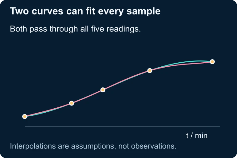Separated measurements leave the behavior between samples undetermined. Two differentiable curves can pass through the same readings while having different derivatives between them.

SECTION 8

Connections to Advanced Topics

Estimating limits from tables is your entry point into the broader landscape of limit evaluation. As you progress through AP Calculus AB, you will encounter algebraic and analytic methods that complement and extend the numerical approach. The table below maps the journey from table-based estimation to more advanced techniques.

Table-Based Estimation	Advanced Technique	When to Use
Observe outputs stabilizing near L	Direct substitution	When f is continuous at c; simply compute f(c)
Detect 0/0 form from table behavior	Algebraic simplification	Factor, cancel, then substitute (as in the worked example)
Table suggests finite L despite 0/0	L'Hôpital's Rule	For indeterminate forms 0/0 or ∞/∞ (covered later in the course)
Left and right outputs squeeze toward the same L	Squeeze Theorem	Bounding f between two functions that share the same limit at c
Graph corroborates table estimate	Graphical estimation	Visual check from the graph of f; often used alongside tables on the AP exam

How table-based estimation connects to more advanced limit evaluation techniques.

The formal epsilon-delta definition of a limit, which you may encounter in a college calculus course, provides the logical backbone for everything the table suggests numerically. In that framework, for every tolerance ε > 0 on the output, there exists a closeness requirement δ > 0 on the input such that |f(x) − L| < ε whenever 0 < |x − c| < δ. Each row of your table is, in effect, a single (δ, ε) witness pair—a concrete demonstration that the outputs remain near L when the inputs are near c. Mastering table-based estimation now will give you deep conceptual preparation for that formalism.

SECTION 9

Practice Problems

Question 1: CONCEPTUAL

A table of values shows f(1.9) = 4.8, f(1.99) = 4.98, f(1.999) = 4.998, and f(2.1) = 5.2, f(2.01) = 5.02, f(2.001) = 5.002. However, f(2) = 7. Which of the following is the best estimate for lim x→2 f(x)?

A. 7
B. 5
C. 4.998
D. 5.002
E. The limit does not exist.

Show answer (B)

The correct answer is B. The limit depends on the trend of f(x) as x approaches 2, not the value at x = 2 itself. From the left, outputs approach 5 (4.8, 4.98, 4.998 → 5). From the right, outputs also approach 5 (5.2, 5.02, 5.002 → 5). Since both one-sided limits converge to 5, lim x→2 f(x) = 5. Choice A (7) confuses f(2) with the limit. Choices C and D are individual table entries, not the limit itself. Choice E is incorrect because the one-sided limits agree.

Question 2: BASIC CALCULATION

Use the table below to estimate lim x→0 (sin x)/x. x: −0.1 −0.01 −0.001 0.001 0.01 0.1 f(x): 0.99833 0.99998 1.00000 1.00000 0.99998 0.99833 What is the estimated limit?

A. 0
B. 0.99833
C. 1
D. 0.99998
E. The limit does not exist.

Show answer (C)

The correct answer is C. From the left, f(x) values are 0.99833, 0.99998, 1.00000—clearly approaching 1. From the right, f(x) values are 1.00000, 0.99998, 0.99833—also approaching 1. Both one-sided limits converge to 1, so lim x→0 (sin x)/x = 1. This is one of the most important limits in calculus. Choice A (0) might result from incorrectly substituting sin(0)/0 = 0/0 and guessing zero. Choices B and D are individual data points that are close to but not equal to the limit. Choice E is wrong because the convergence is clear and consistent.

Question 3: INTERMEDIATE

The table below gives selected values of a function g(x) near x = 4. x: 3.5 3.9 3.99 3.999 | 4.001 4.01 4.1 4.5 g(x): 2.25 2.81 2.9801 2.998 | 3.002 3.0201 3.21 4.25 Which of the following statements is best supported by the data?

A. lim x→4 g(x) = 3 and g is continuous at x = 4
B. lim x→4 g(x) = 3, but we cannot determine continuity from the table alone
C. lim x→4⁻ g(x) = 2.998 and lim x→4⁺ g(x) = 3.002
D. The limit does not exist because the table does not include g(4).
E. lim x→4 g(x) = 4.25

Show answer (B)

The correct answer is B. From the left, g(x) approaches 3: values 2.25 → 2.81 → 2.9801 → 2.998 converge toward 3. From the right, g(x) also approaches 3: values 3.002 → 3.0201 → 3.21 → 4.25 decrease toward 3 as x nears 4. Both one-sided limits equal 3, so lim x→4 g(x) = 3. However, continuity at x = 4 requires g(4) = 3, and the table provides no value for g(4), so we cannot confirm continuity. Choice A incorrectly claims continuity. Choice C confuses table entries with limits—2.998 and 3.002 are approximations at specific x-values, not the one-sided limits themselves. Choice D is wrong because limits do not require the function to be defined at the point. Choice E uses the value at x = 4.5, far from the target.

Question 4: APPLIED

5 pts

A chemical reaction's concentration C(t) (in mol/L) is measured at times near t = 5 seconds, but the sensor malfunctions at exactly t = 5. t (sec): 4.0 4.5 4.9 4.99 4.999 | 5.001 5.01 5.1 5.5 6.0 C(t): 1.200 1.350 1.470 1.494 1.4994 | 1.5006 1.506 1.530 1.650 1.800 (a) Estimate lim t→5 C(t). Justify your answer using values from both sides of t = 5. (b) The sensor records C(5) = 0.000. Is C continuous at t = 5? Explain. (c) Estimate the average rate of change of C over [4.99, 5.01] and explain its physical meaning.

Show answer

Point 1 (1 pt): From the left, C(t) → 1.5: values 1.200, 1.350, 1.470, 1.494, 1.4994 increasingly approach 1.5. From the right, C(t) → 1.5: values 1.5006, 1.506, 1.530, 1.650, 1.800 decrease toward 1.5 as t → 5⁺. Both one-sided limits converge to 1.5. Point 2 (1 pt): Therefore lim t→5 C(t) = 1.500 mol/L. Point 3 (1 pt): For continuity at t = 5, three conditions must hold: (i) C(5) is defined, (ii) lim t→5 C(t) exists, (iii) lim t→5 C(t) = C(5). Here C(5) = 0.000 but lim t→5 C(t) = 1.5, so condition (iii) fails. C is not continuous at t = 5; the sensor malfunction creates a removable discontinuity. Point 4 (1 pt): Average rate of change over [4.99, 5.01] = [C(5.01) − C(4.99)] / [5.01 − 4.99] = (1.506 − 1.494) / 0.02 = 0.012 / 0.02 = 0.6 mol/(L·sec). Point 5 (1 pt): This rate estimates the instantaneous rate of change of concentration at t = 5 seconds—approximately 0.6 mol/(L·sec)—meaning the concentration is increasing at roughly 0.6 moles per liter per second at that moment.

Question 5: CRITICAL THINKING

3 pts

A student constructs a table to estimate lim x→0 f(x) where f(x) = x · sin(1/x). The student's table uses x = 0.1, 0.01, 0.001, and 0.0001, obtaining f(x) values of approximately 0.0544, −0.00507, 0.000827, and −0.0000306. (a) Based on this table alone, can the student confidently conclude that the limit exists? Justify your reasoning. (b) Use the Squeeze Theorem to determine lim x→0 x · sin(1/x) and explain why the table evidence, while suggestive, is insufficient as a proof.

Show answer

Point 1 (1 pt): The table values alternate in sign (0.0544, −0.00507, 0.000827, −0.0000306) but their magnitudes decrease toward 0. The student can reasonably conjecture that the limit is 0, but the oscillating signs and the fact that only right-hand values were tested mean the evidence is not conclusive. One-sided data alone cannot establish a two-sided limit, and oscillation could signal DNE for a less well-behaved function. Point 2 (1 pt): By the Squeeze Theorem: since −1 ≤ sin(1/x) ≤ 1 for all x ≠ 0, multiplying through by |x| yields −|x| ≤ x · sin(1/x) ≤ |x|. As x → 0, both −|x| → 0 and |x| → 0, so by the Squeeze Theorem, lim x→0 x · sin(1/x) = 0. Point 3 (1 pt): The table evidence is suggestive because the magnitudes of f(x) shrink, but it is insufficient as a proof for two reasons: (i) a finite number of data points cannot rule out pathological behavior between the sampled values, and (ii) the Squeeze Theorem provides a rigorous, airtight argument covering all x near 0—not merely a discrete sample. This example illustrates why algebraic/analytic confirmation is essential after numerical estimation.

SUMMARY

Summary

Estimating limits from tables is a foundational skill in AP Calculus AB. To apply the method, select x-values that approach the target point c from both sides, compute f(x) at each, and observe whether the outputs converge to a single value L. The left-hand limit and right-hand limit must agree for the two-sided limit to exist. Remember that the value of f at c is irrelevant to the limit—only the trend of nearby values matters.

Watch for four key patterns: convergence (limit exists), one-sided disagreement (limit DNE), unbounded growth (outputs → ±∞), and oscillation (no settling). Use powers-of-ten spacing (c ± 0.1, 0.01, 0.001, …) to expose convergence patterns clearly. Finally, treat table estimates as a starting hypothesis and, when possible, confirm with algebraic simplification or the Squeeze Theorem.