

SECTION 1
Historical Context & Motivation
The quest to understand instantaneous change stretches back to antiquity, but the formal tools for measuring it crystallized only over several centuries. Ancient Greek geometers such as Archimedes computed tangent lines to specific curves—most famously the spiral that bears his name—by clever geometric arguments that amounted to finding slopes at individual points. These early efforts showed that the idea of local rate of change was both natural and useful, even before a general calculus existed.
During the 17th century, mathematicians like Fermat, Barrow, and Descartes developed algebraic techniques for tangent lines, effectively computing what we now call difference quotients and then letting the interval shrink toward zero. Newton and Leibniz independently formalized these ideas into the differential calculus, yet the numerical estimation of derivatives—using tables of data or discrete measurements—remained a central practical skill in astronomy, navigation, and engineering long before analytic differentiation rules were catalogued.
c. 250 BCE • Archimedes' Tangent Lines
1637 • Fermat's Method of Adequality
1684–1687 • Newton & Leibniz Formalize Calculus
1936 • Richardson's Numerical Differentiation
The central question that motivates this lesson is deceptively simple: if you cannot find an algebraic derivative—perhaps the function is defined only by a data table, a graph, or a complicated expression—how can you still approximate the instantaneous rate of change at a specific point? The answer lies in the very definition of the derivative as a limit of difference quotients, and the practical art of choosing intervals wisely.
SECTION 2
Core Principles & Definitions
Estimating derivatives at a point rests on a handful of interconnected ideas. The formal derivative f′(a) is defined as the limit of slopes of secant lines through (a, f(a)) and a nearby point as the nearby point approaches a. When we estimate rather than compute that limit exactly, we choose a small but nonzero interval and compute the corresponding difference quotient. The smaller the interval, the closer our estimate tends to be—provided the function is smooth enough near a.
Difference Quotient
Forward, Backward & Symmetric Differences
Secant Line Interpretation
Table & Graph Estimation
KEY TAKEAWAY
SECTION 3
Visual Explanation — Secant to Tangent
The diagram below illustrates the geometric heart of derivative estimation. A smooth curve y = f(x) passes through the point P = (a, f(a)). Two secant lines are drawn: one connecting P to a relatively distant point Q₁, and another connecting P to a much closer point Q₂. As the second point slides toward P, the secant line rotates toward the tangent line, whose slope is f′(a). The corresponding difference quotients converge to the derivative.
Notice that the secant through the closer pair of points (green, dashed) is nearly parallel to the tangent (solid cyan). In practice, when we lack an analytic formula and must estimate f′(a), we pick the smallest available interval around a and compute the corresponding slope. The visual confirms the guiding intuition: smaller intervals produce better approximations.
SECTION 4
Mathematical Framework
Three standard difference quotient formulas serve as the primary tools for estimating a derivative numerically. Each arises from choosing which neighboring point(s) to pair with a. Understanding how they relate to one another—and why the symmetric form tends to be more accurate—is essential for the AP exam.
FORWARD DIFFERENCE QUOTIENT
Uses a point to the right of a. The error is proportional to h (first-order accuracy).
BACKWARD DIFFERENCE QUOTIENT
Uses a point to the left of a. Also first-order accurate, with comparable error magnitude.
SYMMETRIC (CENTRAL) DIFFERENCE QUOTIENT
Averages information from both sides of a. The error is proportional to h², making this second-order accurate—often significantly better for the same step size.
To see why the central difference is superior, consider the Taylor expansion of f(a + h) and f(a − h). When these are subtracted, the even-powered error terms cancel, leaving an error of order h² rather than h. On the AP exam, when a table of values gives data on both sides of a, always prefer the symmetric difference quotient unless the problem specifically directs otherwise.
DERIVATIVE AS A LIMIT
This is the formal definition. Estimation replaces the limit with a small but nonzero value of h, accepting a controlled approximation error.
AP Exam Tip
SECTION 5
Comparing Estimation Methods
The three difference quotient methods are not created equal, and the choice among them often depends on which data points are available. The diagram below visualizes how the forward, backward, and symmetric estimates relate to the true tangent slope for a concave-up function. Observe how the central difference (green) bisects the gap between the forward and backward secant slopes, landing closer to the tangent.
| Method | Formula | Data Needed | Error Order |
|---|---|---|---|
| Forward | [f(a + h) − f(a)] / h | f(a) and f(a + h) | O(h) |
| Backward | [f(a) − f(a − h)] / h | f(a − h) and f(a) | O(h) |
| Central (Symmetric) | [f(a + h) − f(a − h)] / (2h) | f(a − h) and f(a + h) | O(h²) |
Summary of three finite-difference derivative estimations
The table confirms the key advantage of the central difference: its error shrinks quadratically with h, so halving the interval reduces error by roughly a factor of four instead of two. For concave-up functions, the forward estimate overshoots and the backward estimate undershoots the true derivative; the reverse is true for concave-down functions. Recognizing this pattern helps you judge whether your estimate is an over- or under-approximation, a frequent question on the AP exam.
SECTION 6
Worked Example
Consider the following table of values for a differentiable function g, which gives the temperature (in °C) of a chemical reaction at selected times t (in minutes).
| t (min) | g(t) (°C) |
|---|---|
| 0 | 22 |
| 3 | 31 |
| 5 | 40 |
| 8 | 53 |
| 12 | 59 |
Temperature data for the worked example
Estimate g′(5) using the data in the table. Include units.
Estimating g′(5) from Tabular Data
- 1
Step 1 — Identify the target and nearest data points
We want f′(5). The table gives g(5) = 40, with neighboring values g(3) = 31 (to the left) and g(8) = 53 (to the right). Since we have data on both sides of t = 5, the symmetric (central) difference quotient is the best choice. - 2
Step 2 — Apply the symmetric difference quotient
g′(5) ≈ [g(8) − g(3)] / (8 − 3) = [53 − 31] / 5 = 22 / 5. - 3
Step 3 — Simplify and attach units
g′(5) ≈ 22 / 5 = 4.4. Because g is measured in °C and t in minutes, the derivative carries units of °C per minute.g′(5) ≈ 4.4 °C/min - 4
Step 4 — Interpret the result
At t = 5 minutes, the temperature of the reaction is increasing at approximately 4.4 degrees Celsius per minute. This is an approximation because the data points are not infinitesimally close to t = 5; the actual rate could differ slightly.
Why Not Use t = 5 and t = 8?
 Using readings on both sides of 5 minutes gives a secant estimate of 4.4 °C/min. The times are unequally spaced, so the estimate uses their actual time difference.
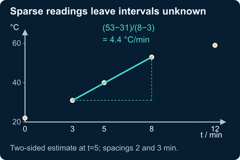 Using readings on both sides of 5 minutes gives a secant estimate of 4.4 °C/min. The times are unequally spaced, so the estimate uses their actual time difference.
SECTION 7
Strengths, Limitations & Common Pitfalls
Derivative estimation from data or graphs is an indispensable tool, but it carries inherent trade-offs. Understanding these trade-offs will help you earn full credit on the AP exam and avoid common errors that lead to point deductions.
| Strengths | Limitations |
|---|---|
| Works with purely numerical or graphical data—no formula needed. | Accuracy depends on interval size; large h values yield coarse estimates. |
| Central difference provides second-order accuracy with minimal computation. | If data is only available on one side of a, you cannot form a symmetric quotient. |
| Gives physical insight—units of the derivative emerge naturally from the quotient. | Cannot detect rapid local oscillations between data points; the estimate smooths them out. |
| Straightforward to apply under time pressure during an exam. | Unequal spacing in a table means you must be careful to use the correct Δx in the denominator. |
Strengths vs. Limitations of numerical derivative estimation
COMMON PITFALL
SECTION 8
Connection to the Formal Derivative & Advanced Topics
Estimating derivatives is not merely a test-prep technique—it is the conceptual bridge between the informal notion of 'slope at a point' and the rigorous limit definition of the derivative. Mastering estimation deepens your understanding of what f′(a) truly represents and prepares you for several more advanced ideas you will encounter later in the course and beyond.
| This Lesson (Estimation) | Formal / Advanced Extension |
|---|---|
| Difference quotient with finite h | Limit definition f′(a) = lim(h→0) [f(a+h) − f(a)] / h |
| Choosing the smallest available h | Epsilon-delta formalization of limits (Calc BC / Real Analysis) |
| Central difference O(h²) accuracy | Higher-order finite difference schemes in Numerical Analysis |
| Estimating f′ from a table | Numerical ODE solvers (Euler's method uses the same idea in reverse) |
| Over/underestimates linked to concavity | The second derivative test and error bounds in Taylor polynomials |
How estimation connects to formal derivatives and advanced topics
In particular, the observation that concavity determines whether a linear approximation overestimates or underestimates a function reappears when you study linearization and Taylor polynomial error bounds later in the AP Calculus AB curriculum. Euler's method for solving differential equations, which appears in BC and is previewed in some AB courses, literally uses the forward difference quotient in reverse—stepping along a curve using estimated slopes. Mastering estimation now lays the groundwork for all of these topics.
SECTION 9
Practice Problems
Question 1: CONCEPTUAL
- A. Greater than f′(4)
- B. Less than f′(4)
- C. Equal to f′(4)
- D. It depends on the sign of f′(4)
- E. It cannot be determined without more information
Show answer (B)
Question 2: BASIC CALCULATION
- A. 11.83
- B. 12.00
- C. 12.01
- D. 12.61
- E. 12.06
Show answer (C)
Question 3: INTERMEDIATE
- A. 4.6
- B. 5.2
- C. 5.8
- D. 5.0
- E. 6.5
Show answer (B)
Question 4: APPLIED
5 ptsShow answer
Question 5: CRITICAL THINKING
4 ptsShow answer
SUMMARY
Lesson Summary
Summary
When an analytic formula is unavailable or impractical, you can estimate the derivative f′(a) by computing a difference quotient—the slope of a secant line through two nearby points on the curve. Three standard forms exist: the forward difference [f(a + h) − f(a)] / h, the backward difference [f(a) − f(a − h)] / h, and the symmetric (central) difference [f(a + h) − f(a − h)] / (2h). The central difference is generally the most accurate because its error is proportional to h² rather than h.
When working from a table, always identify the two data points closest to and flanking the target x-value and form the symmetric quotient. Remember that concavity determines whether a one-sided estimate is an overestimate or underestimate: concave up means forward overshoots and backward undershoots, while concave down reverses this pattern. Always include units and a contextual interpretation when the problem involves a real-world scenario.