Determining Concavity of Functions over Their Domains - AP Calculus AB

SECTION 1

Historical Context & Motivation

The study of curvature and the shape of curves predates modern calculus itself, yet it was the systematic development of differentiation that gave mathematicians the precise tools to describe how a function bends. Ancient Greek geometers, particularly Apollonius of Perga, studied the properties of conic sections and recognized that parabolas and hyperbolas curve in fundamentally different ways. However, they lacked an algebraic framework to generalize these observations to arbitrary functions. The concept of concavity — whether a curve opens upward or downward at a given point — remained intuitive and geometric until the invention of calculus in the seventeenth century.

~200 BCE • Apollonius and Conic Sections

Apollonius of Perga systematically classified conic sections, noting their curvature properties and laying geometric groundwork for later analysis of how curves bend.

1684 • Leibniz Publishes Differential Calculus

Gottfried Wilhelm Leibniz published his foundational work on the calculus, introducing the notation dy/dx and enabling systematic computation of rates of change.

1736 • Euler's Method of Fluxions

Leonhard Euler formalized the use of higher-order derivatives, recognizing that the second derivative captures how the slope itself is changing — the essence of concavity.

1797 • Lagrange's Théorie des Fonctions

Joseph-Louis Lagrange attempted to place calculus on an algebraic footing, clearly articulating the role of the second derivative in classifying the shape of function graphs near critical points.

1821 • Cauchy Rigorous Analysis

Augustin-Louis Cauchy provided rigorous epsilon-delta definitions that formalized continuity and differentiability, completing the theoretical framework for the concavity test used today.

The central question that concavity analysis answers is deceptively simple: given a function that is increasing, how is it increasing? Is the rate of increase itself growing (accelerating upward), or is the rate of increase diminishing (decelerating)? A first derivative alone cannot distinguish between these two scenarios — it tells you the slope but not whether the slope is getting steeper or flatter. This gap is precisely what the second derivative, and the formal notion of concavity, fills.

SECTION 2

Core Principles & Definitions

Concavity describes the direction in which a curve bends. To make this precise, we connect the geometric picture — the shape of the graph — to the analytical behavior of derivatives. Before diving into calculations, it is essential to internalize the four foundational ideas that underpin concavity analysis.

Concave Up

A function f is concave up on an interval if, for every point in that interval, the graph lies above all of its tangent lines. Equivalently, f′ is increasing on that interval. Visually, the curve opens upward like a cup.

Concave Down

A function f is concave down on an interval if, for every point in that interval, the graph lies below all of its tangent lines. Equivalently, f′ is decreasing on that interval. Visually, the curve opens downward like a frown.

The Second Derivative Test for Concavity

If f″(x) > 0 on an interval, then f is concave up there. If f″(x) < 0 on an interval, then f is concave down there. The sign of the second derivative directly reveals concavity.

Inflection Points

A point of inflection is where the concavity changes — from concave up to concave down or vice versa. At such a point, f″ equals zero or is undefined, and the sign of f″ must change on either side.

✦

KEY TAKEAWAY

Think of driving along a winding mountain road. The first derivative is your speedometer — it tells you how fast you're going. The second derivative is the feeling in your seat: if you're being pushed back (accelerating), the road is concave up; if you're lurching forward (decelerating), it is concave down. The moment you switch between these feelings is an inflection point.

A critical subtlety: f″(c) = 0 is a necessary condition for a point of inflection at x = c (when f″ exists there), but it is not sufficient. The function f(x) = x⁴ satisfies f″(0) = 0, yet x = 0 is not an inflection point because f″ does not change sign — f″(x) = 12x² ≥ 0 everywhere. You must always verify a sign change in f″ across the candidate point.

SECTION 3

Visual Explanation of Concavity

The diagram below shows a cubic function, f(x) = x³ − 3x, alongside its second derivative f″(x) = 6x. The shading on the graph of f indicates the concavity regions: cyan shading marks where the function is concave up (f″ > 0), and pink shading marks where it is concave down (f″ < 0). The inflection point where concavity changes is indicated at the origin.

The graph of f(x) = x³ − 3x is shown in violet. The pink-shaded region (x < 0) marks where f is concave down, and the cyan-shaded region (x > 0) marks where f is concave up. The amber dot at the origin marks the inflection point where concavity changes.

Notice how the tangent lines on the left side of the graph (where x < 0) lie above the curve — the graph sags below its tangent lines, which is the geometric definition of concave down. On the right side (where x > 0), tangent lines lie below the curve, meaning the graph arches above them — the hallmark of concave up. At the origin, the tangent line actually crosses through the curve, reflecting the transition in concavity. This crossing behavior at an inflection point is one of the most reliable visual signatures you can look for.

A walking path crosses a ridge and hollow beside a staff-bearing observer. For f(x) = x³ − 3x, height, slope, and change in slope are different quantities. The extrema occur at x = −1 and 1; concavity changes at x = 0.

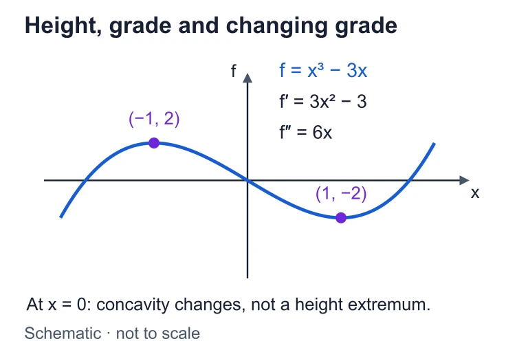For f(x) = x³ − 3x, height, slope, and change in slope are different quantities. The extrema occur at x = −1 and 1; concavity changes at x = 0.

SECTION 4

Mathematical Framework

The formal mathematical machinery for determining concavity rests on the relationship between a function, its first derivative, and its second derivative. Each derivative adds a layer of information: f tells you position, f′ tells you slope (direction of motion), and f″ tells you the rate of change of slope (curvature). The following equations and definitions make this precise.

CONCAVE UP CONDITION

f″(x) > 0 on (a, b) ⟹ f is concave up on (a, b)

If the second derivative is positive throughout an open interval, then the first derivative f′ is increasing on that interval, meaning the slopes of the tangent lines are getting steeper from left to right. The graph curves upward.

CONCAVE DOWN CONDITION

f″(x) < 0 on (a, b) ⟹ f is concave down on (a, b)

If the second derivative is negative throughout an open interval, then f′ is decreasing, meaning tangent-line slopes are getting less steep (or more negative). The graph curves downward.

INFLECTION POINT CRITERION

f″(c) = 0 or f″(c) DNE, and f″ changes sign at x = c

A candidate for an inflection point is any x = c in the domain of f where f″(c) = 0 or f″(c) does not exist. To confirm it is an inflection point, you must verify that f″ changes from positive to negative (or vice versa) as x passes through c.

The Procedure for Determining Concavity

Step 1: Compute f″(x), the second derivative of the given function.
Step 2: Find all values of x where f″(x) = 0 or f″(x) does not exist. These are the candidate partition points.
Step 3: Use the candidate points to divide the domain into test intervals.
Step 4: Evaluate f″ at a test value in each interval. If f″ > 0, the function is concave up on that interval; if f″ < 0, concave down.
Step 5: Identify inflection points where f″ changes sign, provided f is continuous at those x-values.

⚠

Common Pitfall

Students frequently assume that f″(c) = 0 automatically makes x = c an inflection point. Remember: f(x) = x⁴ has f″(0) = 0 but is concave up everywhere (f″(x) = 12x² ≥ 0). The sign-change test is non-negotiable.

SECTION 5

Sign Charts & Interval Classification

A sign chart for f″ is the single most efficient organizational tool for concavity analysis on the AP Calculus AB exam. It provides a complete visual summary of where the second derivative is positive, negative, or zero, and therefore where the original function is concave up, concave down, or has an inflection point. The diagram below illustrates the sign chart approach for the function f(x) = 3x⁵ − 20x³, whose second derivative is f″(x) = 60x³ − 120x = 60x(x² − 2).

The sign chart for f″(x) = 60x(x² − 2) partitions the number line at x = −√2, 0, and √2. Each interval is tested to determine the sign of f″, from which concavity and inflection points are directly read. All three candidate points are confirmed inflection points because f″ changes sign at each.

To construct this chart, we first factored f″(x) = 60x(x − √2)(x + √2), identified the zeros at x = −√2, 0, and √2, and then picked one test value in each of the four resulting intervals. Because the sign of f″ alternates across every partition point, all three candidates are genuine inflection points. The AP exam frequently tests your ability to read such sign charts and translate them into statements about the original function's shape.

💡

Exam Strategy

On free-response questions, clearly label your sign chart with the sign of f″ in each interval and explicitly state the concavity conclusion. Writing "f″(x) > 0 on (−√2, 0), so f is concave up on (−√2, 0)" earns credit; merely stating "concave up" without justification typically does not.

SECTION 6

Worked Example

Let us work through a complete concavity analysis for a function typical of what appears on the AP Calculus AB exam. We will determine all intervals of concavity and identify all inflection points for f(x) = x⁴ − 6x² + 8x + 1.

Determine Concavity and Inflection Points for f(x) = x⁴ − 6x² + 8x + 1

1
Step 1 — Compute the First Derivative

Using the power rule term by term: f′(x) = 4x³ − 12x + 8. While we do not directly need f′ for the concavity test, computing it first confirms we are differentiating correctly and prepares us for the second derivative.

f′(x) = 4x³ − 12x + 8
2
Step 2 — Compute the Second Derivative

Differentiate f′(x) again: f″(x) = 12x² − 12. Factor out the common factor: f″(x) = 12(x² − 1) = 12(x − 1)(x + 1).

f″(x) = 12(x − 1)(x + 1)
3
Step 3 — Find Candidate Points

Set f″(x) = 0: 12(x − 1)(x + 1) = 0 gives x = −1 and x = 1. Since f″ is a polynomial, it exists everywhere, so there are no points where f″ is undefined. The domain of f is all real numbers, so both candidates lie within the domain.

Candidates: x = −1, x = 1
4
Step 4 — Build the Sign Chart

The candidates partition ℝ into three intervals: (−∞, −1), (−1, 1), and (1, ∞). Test x = −2 in the first interval: f″(−2) = 12(−2 − 1)(−2 + 1) = 12(−3)(−1) = 36 > 0. Test x = 0 in the second interval: f″(0) = 12(0 − 1)(0 + 1) = 12(−1)(1) = −12 < 0. Test x = 2 in the third interval: f″(2) = 12(2 − 1)(2 + 1) = 12(1)(3) = 36 > 0.

f″ > 0 on (−∞, −1) ∪ (1, ∞); f″ < 0 on (−1, 1)
5
Step 5 — State Concavity and Inflection Points

Since f″ > 0 on (−∞, −1), the function is concave up there. Since f″ < 0 on (−1, 1), the function is concave down there. Since f″ > 0 on (1, ∞), the function is concave up there. At x = −1, f″ changes from positive to negative: inflection point at (−1, f(−1)) = (−1, (−1)⁴ − 6(−1)² + 8(−1) + 1) = (−1, 1 − 6 − 8 + 1) = (−1, −12). At x = 1, f″ changes from negative to positive: inflection point at (1, f(1)) = (1, 1 − 6 + 8 + 1) = (1, 4).

Concave up on (−∞, −1) ∪ (1, ∞). Concave down on (−1, 1). Inflection points at (−1, −12) and (1, 4).

SECTION 7

Common Errors & How to Avoid Them

Concavity analysis is conceptually straightforward, but several recurring errors cause students to lose points on the AP exam. Recognizing these pitfalls in advance is one of the most effective ways to improve your accuracy and earn full credit.

Common Error	Why It's Wrong	Correct Approach
Claiming f″(c) = 0 guarantees an inflection point	f″(c) = 0 is necessary (when f″ exists) but not sufficient. f(x) = x⁴ has f″(0) = 0 but no inflection point.	Always verify a sign change in f″ across the candidate point.
Confusing concavity with increasing/decreasing	Increasing/decreasing is determined by f′. A function can be increasing and concave down simultaneously (e.g., ln x for x > 1).	Use f′ for monotonicity questions and f″ for concavity questions. Keep these analyses separate.
Ignoring points where f″ does not exist	Concavity can change at a point where f″ is undefined. For f(x) = $x^{1/3}$ , f″(0) DNE but the concavity changes.	Include in your candidate list all x where f″ = 0 OR f″ DNE, provided x is in the domain of f.
Reporting intervals in the wrong format	Concavity is an open-interval property. Writing "concave up on [−1, 1]" is technically imprecise because concavity is defined on open intervals.	Use open interval notation: (a, b). On the AP exam, either open or closed intervals are accepted when the function is continuous at the endpoints, but open is standard practice.

Common concavity analysis errors and their corrections

✦

KEY TAKEAWAY

Think of an inflection point like a gearshift in a car. Just because you release the gas (f″ = 0) doesn't mean you've shifted gears — you might just be coasting in the same gear. To confirm a genuine shift in concavity, you need to check that the car actually transitions from accelerating to decelerating (or vice versa). The sign-change test is how you verify that the shift actually occurred.

SECTION 8

Connection to the Second Derivative Test and Beyond

Concavity analysis is not an isolated skill — it connects directly to several other important topics in AP Calculus AB and provides a foundation for more advanced ideas you may encounter in future courses. The most immediate application is the Second Derivative Test for Local Extrema, which uses concavity at a critical point to determine whether that point is a local maximum or minimum without needing a first-derivative sign chart.

Concept	Concavity Analysis (This Lesson)	Advanced Extension
Classifying critical points	If f′(c) = 0 and f″(c) > 0, then f has a local min at c. If f″(c) < 0, local max.	Higher-order derivative test: if f″(c) = 0, examine f‴(c), f⁽⁴⁾(c), etc. (Calculus BC / multivariable)
Curve sketching	Concavity intervals + inflection points combined with increasing/decreasing analysis produce a complete sketch.	Curvature κ = \|f″\|/(1 + (f′)²)^(3/2) gives a quantitative measure of bending (multivariable calculus).
Optimization	f″ > 0 on an interval ensures f is concave up, guaranteeing that any critical point there is a global min on that interval.	Convex optimization (convex = concave up everywhere) guarantees every local min is a global min — foundational in machine learning.
Motion problems	If s(t) is position, s″(t) = a(t) is acceleration. Concavity of s tells you the direction of acceleration.	In physics, the third derivative (jerk) measures the rate of change of acceleration — extending the concavity idea one level further.

How concavity analysis connects to broader calculus topics

Understanding concavity deeply prepares you not only for the AP exam but also for multivariable calculus, differential equations, and applied optimization. In economics, a concave-down production function reflects diminishing returns; in physics, concavity of a position-time graph distinguishes constant acceleration from deceleration. Mastering the second derivative's role in determining shape is one of the most transferable skills in your calculus toolkit.

SECTION 9

Practice Problems

Question 1: CONCEPTUAL

If f″(x) > 0 for all x in the interval (2, 5), which of the following must be true about the graph of f on (2, 5)?

A. f is increasing on (2, 5).
B. f is concave up on (2, 5).
C. f has a local minimum in (2, 5).
D. f has an inflection point in (2, 5).
E. f′ is concave up on (2, 5).

Show answer (B)

Correct Answer: B. By definition, f″(x) > 0 on an interval means f is concave up on that interval. (A) is wrong because f″ > 0 tells us f′ is increasing, not that f itself is increasing — f could be decreasing with an increasing slope (like the right branch of a parabola opening upward below the x-axis). (C) is wrong because a local minimum requires f′ = 0 with a sign change in f′, which is not guaranteed. (D) is wrong because inflection points require a change in the sign of f″, which contradicts f″ > 0 throughout. (E) confuses levels of analysis — f″ > 0 means f′ is increasing, but says nothing about the concavity of f′ (which would require f‴).

Question 2: BASIC CALCULATION

Determine the intervals on which f(x) = x³ − 6x² + 9x + 2 is concave up and concave down.

A. Concave up on (−∞, 2); concave down on (2, ∞)
B. Concave up on (2, ∞); concave down on (−∞, 2)
C. Concave up on (−∞, 1) ∪ (3, ∞); concave down on (1, 3)
D. Concave up on (−∞, ∞)
E. Concave up on (−∞, 2); concave down on (2, ∞), with no inflection point

Show answer (B)

Correct Answer: B. Compute f′(x) = 3x² − 12x + 9 and f″(x) = 6x − 12 = 6(x − 2). Setting f″(x) = 0 gives x = 2. For x < 2 (test x = 0): f″(0) = 6(0) − 12 = −12 < 0, so f is concave down on (−∞, 2). For x > 2 (test x = 3): f″(3) = 6(3) − 12 = 6 > 0, so f is concave up on (2, ∞). Since f″ changes sign at x = 2, there is an inflection point at (2, f(2)) = (2, 4). (A) reverses the concavity intervals. (C) uses the zeros of f′, not f″ — a classic mix-up. (D) incorrectly claims concave up everywhere. (E) gets the concavity intervals reversed and also claims no inflection point even though f″ changes sign at x = 2.

Question 3: INTERMEDIATE

Let g(x) =

xe^{−x}

. Find all inflection points of g and determine the intervals of concavity.

A. Inflection point at x = 1; concave down on (−∞, 1), concave up on (1, ∞)
B. Inflection point at x = 2; concave up on (−∞, 2), concave down on (2, ∞)
C. Inflection point at x = 2; concave down on (−∞, 2), concave up on (2, ∞)
D. Inflection points at x = 0 and x = 2; concave up on (0, 2)
E. No inflection points; concave down on (−∞, ∞)

Show answer (C)

Correct Answer: C. Using the product rule: g′(x) =

e^{−x}

−

xe^{−x}

= (1 − x)

e^{−x}

. Differentiating again: g″(x) = d/dx[(1 − x)

e^{−x}

] = (−1)

e^{−x}

+ (1 − x)(−

e^{−x}

) = −

e^{−x}

−

e^{−x}

xe^{−x}

= (x − 2)

e^{−x}

. Setting g″(x) = 0: since

e^{−x}

> 0 for all x, we need x − 2 = 0, so x = 2. For x < 2, x − 2 < 0, so g″ < 0 (concave down). For x > 2, x − 2 > 0, so g″ > 0 (concave up). The sign changes at x = 2, confirming an inflection point. (A) incorrectly places the inflection at x = 1, which is where g′ = 0 (the critical point, not inflection). (B) gets the right location but reverses concavity. (D) invents a second inflection point. (E) ignores the sign change entirely.

Question 4: APPLIED

5 pts

A particle moves along the x-axis with position function s(t) = t⁴ − 8t³ + 18t² for t ≥ 0. (a) Find all values of t at which the acceleration of the particle equals zero. (b) Determine the intervals on which the position function s is concave up and concave down for t > 0. (c) At what time(s) does the particle's acceleration change from positive to negative, or vice versa? Explain the physical meaning of these times.

Show answer

Rubric (5 points): Point 1 — Correct second derivative: s′(t) = 4t³ − 24t² + 36t, s″(t) = 12t² − 48t + 36 = 12(t² − 4t + 3) = 12(t − 1)(t − 3). Point 2 — Part (a): Zeros of acceleration: s″(t) = 0 when t = 1 and t = 3. Point 3 — Part (b): Correct concavity intervals with justification: Test t = 0.5: s″(0.5) = 12(0.5 − 1)(0.5 − 3) = 12(−0.5)(−2.5) = 15 > 0 → concave up on (0, 1). Test t = 2: s″(2) = 12(2 − 1)(2 − 3) = 12(1)(−1) = −12 < 0 → concave down on (1, 3). Test t = 4: s″(4) = 12(4 − 1)(4 − 3) = 12(3)(1) = 36 > 0 → concave up on (3, ∞). So s is concave up on (0, 1) ∪ (3, ∞) and concave down on (1, 3). Point 4 — Part (c): Identification of sign changes: At t = 1, acceleration changes from positive to negative. At t = 3, acceleration changes from negative to positive. Point 5 — Physical interpretation: These are the inflection points of the position graph. At t = 1, the particle transitions from accelerating (speed increasing in the direction of motion) to decelerating. At t = 3, the particle transitions back from decelerating to accelerating. These times represent moments when the net force acting on the particle changes direction.

Question 5: CRITICAL THINKING

3 pts

Let f be a twice-differentiable function on (−∞, ∞) such that f″(x) = x²(x − 4). (a) Find all candidates for inflection points of f. (b) Determine which candidates are actually inflection points. Justify your answer using sign analysis. (c) Explain why x = 0 is or is not an inflection point, even though f″(0) = 0.

Show answer

Rubric (3 points): Point 1 — Correct candidates: f″(x) = x²(x − 4) = 0 when x = 0 and x = 4. These are the only candidates since f″ is a polynomial and exists everywhere. Point 2 — Sign analysis and correct identification: Test x = −1: f″(−1) = (1)(−5) = −5 < 0. Test x = 2: f″(2) = (4)(−2) = −8 < 0. Test x = 5: f″(5) = (25)(1) = 25 > 0. The sign chart shows: f″ < 0 on (−∞, 0), f″ < 0 on (0, 4), f″ > 0 on (4, ∞). f″ does NOT change sign at x = 0 (negative on both sides), so x = 0 is NOT an inflection point. f″ DOES change sign at x = 4 (negative to positive), so x = 4 IS an inflection point. Point 3 — Explanation for x = 0: Although f″(0) = 0, the factor x² is always non-negative, so it does not contribute a sign change. The second derivative is negative on both sides of x = 0 (it is negative for x < 0 because x² > 0 and (x − 4) < 0, and negative for 0 < x < 4 for the same reason). Since f″ does not change sign at x = 0, there is no change in concavity, and x = 0 is not an inflection point. This illustrates that f″(c) = 0 is necessary but not sufficient for an inflection point — the sign-change condition is essential.

SUMMARY

Lesson Summary

Summary

Determining the concavity of a function requires analyzing the second derivative f″(x). When f″(x) > 0 on an interval, the function is concave up (the graph lies above its tangent lines and f′ is increasing). When f″(x) < 0 on an interval, the function is concave down (the graph lies below its tangent lines and f′ is decreasing). The systematic procedure involves computing f″, finding where f″ = 0 or DNE, building a sign chart, and testing each resulting interval.

Inflection points occur where f″ changes sign — not merely where f″ equals zero. Always verify the sign change; the condition f″(c) = 0 is necessary but not sufficient. Concavity analysis connects to the Second Derivative Test for local extrema, complete curve sketching, and optimization problems — making it one of the most widely applicable tools in the AP Calculus AB toolkit.