Finding the Area Between Curves Expressed as Functions of y - AP Calculus AB

SECTION 1

Historical Context & Motivation

The problem of measuring the area enclosed by curves has roots stretching back to antiquity, long before the formal invention of calculus. Greek mathematicians such as Archimedes devised the method of exhaustion to approximate areas of parabolic segments by inscribing ever-finer collections of rectangles and triangles. While remarkably powerful for its era, this approach was limited to specific geometric shapes and lacked a general algebraic framework for curves that could not easily be described as functions of a single horizontal variable.

The seventeenth century saw Isaac Newton and Gottfried Wilhelm Leibniz independently formalize integration as the inverse operation of differentiation, giving rise to the Fundamental Theorem of Calculus. Leibniz's notation — the integral sign ∫ and the differential dx or dy — proved especially influential because it made explicit the variable of integration. This notational flexibility revealed that one could compute areas by integrating with respect to y just as naturally as with respect to x, a realization that opened the door to simpler treatments of curves that are more conveniently expressed as horizontal functions of a vertical variable.

~250 BCE • Archimedes' Method of Exhaustion

Archimedes computes the area of a parabolic segment using successively finer polygonal approximations, establishing the conceptual precursor to Riemann sums.

1666–1684 • Newton & Leibniz Develop Calculus

Both mathematicians independently create the framework of differentiation and integration, with Leibniz's ∫ notation allowing explicit choice of the variable of integration (dx or dy).

1854 • Riemann Formalizes the Integral

Bernhard Riemann defines the definite integral rigorously using partitions and limiting sums, giving formal justification to integrating with respect to any variable over an interval.

20th Century • Modern Applications

Engineers, physicists, and economists routinely integrate with respect to y to compute cross-sectional areas, pressure distributions, and consumer surplus — problems where horizontal integration is the natural choice.

Why do we need to integrate with respect to y at all? Consider two curves that, when viewed as functions of x, fail the vertical line test or require splitting the region into multiple sub-integrals. Rewriting those curves as functions of y often collapses the problem into a single, clean integral. The central question this lesson addresses is: how do we set up, evaluate, and interpret such integrals to find the exact area between two curves expressed as x = f(y) and x = g(y)?

SECTION 2

Core Principles & Definitions

Before setting up an area integral with respect to y, it is essential to internalize a few foundational ideas that distinguish this technique from the more familiar integration with respect to x. The same geometric region is being measured in both cases; only the orientation of the representative rectangles and the variable of integration change. Mastering this shift in perspective is one of the most useful skills in applied integration.

Horizontal Representative Rectangles

When integrating with respect to y, each thin rectangle has width Δy (vertical thickness) and length equal to the horizontal distance between the right curve and the left curve at a given y-value.

Right Minus Left

The integrand is always (right function) − (left function), analogous to (top − bottom) when integrating with respect to x. This ensures the integrand remains non-negative across the interval.

Limits of Integration in y

The bounds of the definite integral are the y-coordinates where the two curves intersect. These are found by setting f(y) = g(y) and solving for y.

When to Choose dy Over dx

Prefer integrating with respect to y when the curves are more easily expressed as x = f(y), when integrating with respect to x would require splitting the region into multiple pieces, or when the boundary curves change roles (top/bottom) over the x-interval.

✦

KEY TAKEAWAY

Think of integrating with respect to y like scanning a region with a horizontal laser beam that sweeps from bottom to top. At every height y, the beam measures the horizontal width between the left boundary and the right boundary. Summing all those infinitesimal horizontal strips from the lowest intersection to the highest intersection gives the total enclosed area — much like stacking thin planks side by side to fill a window frame.

SECTION 3

Visual Explanation

The diagram below illustrates the fundamental geometric idea behind integrating with respect to y. Two curves — one serving as the right boundary and the other as the left boundary — enclose a shaded region. Horizontal representative rectangles of width Δy span the gap between the two curves at each height y, and the area is obtained by summing these rectangles from the lower y-bound to the upper y-bound.

The left curve x = g(y) and the right curve x = f(y) enclose a shaded region. Each horizontal rectangle has length f(y) − g(y) and infinitesimal height dy. The total area is the definite integral of these strips from the lower intersection y = c to the upper intersection y = d.

Notice how every horizontal strip extends from the left boundary to the right boundary at a single y-value. This is the key geometric insight: rather than slicing the region into vertical strips (which would require integrating with respect to x and potentially splitting the integral), we use horizontal strips that naturally sweep the entire region in one pass. The shaded gradient in the diagram emphasizes that the area accumulates continuously from y = c to y = d.

SECTION 4

Mathematical Framework

The formal derivation of the area formula when integrating with respect to y mirrors the derivation for integration with respect to x, but with the roles of the axes swapped. We begin by partitioning the y-interval [c, d] into n subintervals, each of width Δy = (d − c)/n. On each subinterval, a horizontal rectangle of height Δy and width f(yᵢ*) − g(yᵢ*) approximates the area of the corresponding horizontal strip. The Riemann sum of these rectangles converges to the definite integral as n → ∞.

RIEMANN SUM APPROXIMATION

A ≈ Σᵢ₌₁ⁿ [f(yᵢ*) − g(yᵢ*)] · Δy

where yᵢ* is a sample point in the i-th subinterval, f(yᵢ*) is the x-value on the right curve, and g(yᵢ*) is the x-value on the left curve.

AREA BETWEEN CURVES (INTEGRATING W.R.T. y)

A = ∫ from c to d [f(y) − g(y)] dy

Here f(y) ≥ g(y) on the interval [c, d], with c and d being the y-coordinates of the intersection points. The integrand f(y) − g(y) represents the horizontal distance between the right and left boundaries at height y.

To apply this formula correctly, follow a systematic procedure. First, express both curves as functions of y — that is, solve for x in terms of y so that you have x = f(y) and x = g(y). Second, determine which curve lies to the right (has the larger x-value) for y-values in the interval; this curve is f(y). Third, find the y-coordinates of all intersection points by solving f(y) = g(y). If the relative positions of the curves switch within the interval, you must split the integral at each crossing point and take absolute values or swap f and g appropriately.

INTERSECTION POINTS

f(y) = g(y) → solve for y = c, y = d

The solutions c and d become the lower and upper limits of integration. If there are more than two intersection points, evaluate the integral over each sub-interval separately.

⚠

Common Pitfall

Students often forget to re-express the curves as functions of y and instead attempt to set up the integral with x-expressions. Always check: if your variable of integration is dy, every function in the integrand must be written in terms of y, and both limits must be y-values.

SECTION 5

Comparing dx and dy Approaches

One of the most important strategic decisions in area-between-curves problems is choosing whether to integrate with respect to x or with respect to y. Both approaches yield the same numerical answer when set up correctly, but one approach is often dramatically simpler than the other. The diagram below illustrates a classic scenario where integrating with respect to y requires only a single integral, whereas integrating with respect to x would force you to split the region and evaluate two or more separate integrals.

Left panel: Vertical strips (dx) require splitting at x₁ because the top/bottom boundaries change. Right panel: Horizontal strips (dy) sweep the entire region in a single integral, making the computation far simpler.

Feature	Integrating w.r.t. x	Integrating w.r.t. y
Strip orientation	Vertical (width dx)	Horizontal (width dy)
Integrand	(top function) − (bottom function)	(right function) − (left function)
Limits of integration	x-coordinates of intersections	y-coordinates of intersections
Best when	Both curves are simple y = f(x) forms and neither changes role	Curves are naturally x = f(y) or dx setup requires splitting
Common pitfall	Forgetting to split when top/bottom roles swap	Forgetting to solve for x as a function of y

Comparison of integration approaches for area between curves

SECTION 6

Worked Example

Let us compute the area of the region enclosed by the curves x = y² and x = y + 2. This is a classic AP Calculus AB problem that is significantly simpler when approached via integration with respect to y.

Finding the Area Between x = y² and x = y + 2

1
Step 1 — Express Both Curves as Functions of y

The curves are already expressed as functions of y. We have x = y² (a rightward-opening parabola) and x = y + 2 (a line with slope 1). No algebraic rearrangement is needed.
2
Step 2 — Find the Intersection Points

Set the two expressions equal: y² = y + 2. Rearranging gives y² − y − 2 = 0, which factors as (y − 2)(y + 1) = 0. The solutions are y = −1 and y = 2. These are the limits of integration.

y = −1 and y = 2
3
Step 3 — Determine Right and Left Curves

Test a value between −1 and 2, say y = 0. For the line: x = 0 + 2 = 2. For the parabola: x = 0² = 0. Since 2 > 0, the line x = y + 2 lies to the right and the parabola x = y² lies to the left throughout the interval [−1, 2].

Integrand: (y + 2) − y²
4
Step 4 — Set Up and Evaluate the Integral

A = ∫ from −1 to 2 [(y + 2) − y²] dy = ∫ from −1 to 2 [y + 2 − y²] dy. Compute the antiderivative: y²/2 + 2y − y³/3. Evaluate at the bounds:
5
Step 5 — Evaluate at Upper Bound y = 2

Substituting y = 2: (2)²/2 + 2(2) − (2)³/3 = 4/2 + 4 − 8/3 = 2 + 4 − 8/3 = 6 − 8/3 = 18/3 − 8/3 = 10/3.

F(2) = 10/3
6
Step 6 — Evaluate at Lower Bound y = −1

Substituting y = −1: (−1)²/2 + 2(−1) − (−1)³/3 = 1/2 − 2 + 1/3 = 3/6 − 12/6 + 2/6 = −7/6.

F(−1) = −7/6
7
Step 7 — Compute the Final Area

A = F(2) − F(−1) = 10/3 − (−7/6) = 10/3 + 7/6 = 20/6 + 7/6 = 27/6 = 9/2.

A = 9/2 square units

💡

Why dy Was Superior Here

Had we integrated with respect to x, we would need to split the region at x = 1 (the vertex of the parabola in x-terms) because for 0 ≤ x ≤ 1 the parabola has two branches (y = √x and y = −√x), while the line has a different domain. The dy approach avoids all of this complexity with a single, clean integral.

SECTION 7

When to Use Each Method — Strengths & Limitations

Choosing the variable of integration is a strategic decision, not a mathematical necessity. Every area problem can theoretically be solved using either dx or dy — the question is which leads to fewer integrals, simpler integrands, and less opportunity for algebraic error. The table below summarizes common problem types and the recommended approach for each.

Scenario	Recommended Approach	Reason
Both curves easily solved for y = f(x), same top/bottom throughout	Integrate w.r.t. x	Direct application; no splitting needed
Curves given as x = f(y) and x = g(y)	Integrate w.r.t. y	Curves are already in the correct form
Top/bottom curves switch roles mid-interval in x	Integrate w.r.t. y	Avoids splitting; one integral instead of two
Sideways parabola (x = ay² + by + c)	Integrate w.r.t. y	Parabola is a single-valued function of y
Both curves are simple polynomials in x	Integrate w.r.t. x	Solving for x in terms of y would be unnecessarily complex

Strategy guide for choosing dx vs. dy

✦

KEY TAKEAWAY

Think of the choice between dx and dy like choosing between two routes to the same destination. A GPS (your mathematical intuition) should evaluate both before committing. If one route has a complicated detour (splitting the integral, inverse functions with ± branches), take the other route. On the AP exam, spending 30 seconds sketching the region and considering both orientations can save several minutes of computation.

SECTION 8

Connection to Advanced Applications

The technique of integrating with respect to y to find area between curves is not an isolated skill — it serves as a gateway to several advanced topics in AP Calculus AB and beyond. Understanding horizontal integration prepares you for volume computations using the shell method (where you integrate cylindrical shells with respect to the axis perpendicular to the axis of rotation) and for setting up double integrals in multivariable calculus where the order of integration matters.

This Lesson's Concept	Advanced Extension
Area = ∫[f(y) − g(y)] dy	Volume via shell method: V = 2π ∫ y · [f(y) − g(y)] dy when revolving about the x-axis
Choosing dy to avoid splitting	Choosing order of integration (dydx vs. dxdy) in double integrals to simplify region bounds
Horizontal representative rectangles	Cross-sectional area functions in volumes of known cross sections
Right − left integrand	Net displacement along the x-axis when velocity is expressed as a function of a vertical parameter

How integration with respect to y connects to advanced topics

Within the AP Calculus AB curriculum specifically, proficiency with dy-integration also appears in free-response questions that ask you to find the area of a region as a precursor to computing its volume when revolved about a vertical line. In such problems, the region definition step is identical to what we have covered in this lesson, and the volume computation simply layers on an additional factor (such as π × [radius]² for the disk/washer method). Building fluency with the area setup now ensures that volume problems feel like a natural extension rather than a new challenge.

SECTION 9

Practice Problems

Question 1: CONCEPTUAL

When computing the area of a region by integrating with respect to y, the integrand is expressed as:

A. (top function) − (bottom function)
B. (right function) − (left function)
C. (upper y-limit) − (lower y-limit)
D. (outer function) − (inner function)
E. (left function) − (right function)

Show answer (B)

The correct answer is B. When integrating with respect to y, horizontal representative rectangles span from the left curve to the right curve, so the integrand is (right function) − (left function). Choice A describes the integrand for integration with respect to x, not y. Choice C confuses the limits of integration with the integrand itself. Choice D uses terminology from polar or washer-method problems, not standard area-between-curves language. Choice E reverses the order, which would yield a negative integrand and an incorrect (negative) area.

Question 2: BASIC CALCULATION

Find the area of the region enclosed by x = y² and x = 4 by integrating with respect to y.

A. 16/3
B. 32/3
C. 8
D. 16
E. 64/3

Show answer (B)

The correct answer is B. Setting y² = 4 gives y = −2 and y = 2. The right curve is x = 4 and the left curve is x = y². The area is A = ∫ from −2 to 2 [4 − y²] dy = [4y − y³/3] from −2 to 2 = (8 − 8/3) − (−8 + 8/3) = (16/3) − (−16/3) = 32/3. Choice A (16/3) is half the answer — a common error from integrating only from 0 to 2 and forgetting the symmetric lower half. Choice C (8) likely results from an incorrect antiderivative. Choice D (16) would be the area of the bounding rectangle 4 × 4, ignoring the parabola. Choice E (64/3) likely stems from an arithmetic error in evaluating the bounds.

Question 3: INTERMEDIATE

Find the area of the region enclosed by x = 2y − y² and x = y² − 4y by integrating with respect to y.

A. 9
B. 27/2
C. 18
D. 27/4
E. 3

Show answer (A)

The correct answer is A. Set 2y − y² = y² − 4y, which simplifies to 6y − 2y² = 0, so 2y(3 − y) = 0, giving y = 0 and y = 3. Test y = 1: 2(1) − 1 = 1 (right) vs. 1 − 4 = −3 (left), so x = 2y − y² is the right curve. The integrand is (2y − y²) − (y² − 4y) = 6y − 2y². Area = ∫ from 0 to 3 (6y − 2y²) dy = [3y² − 2y³/3] from 0 to 3 = 27 − 18 = 9. Choice B (27/2) may arise from doubling the coefficient error. Choice C (18) likely results from forgetting to subtract the left curve. Choice D (27/4) could stem from an integration error. Choice E (3) likely comes from evaluating the integrand at a single point rather than integrating.

Question 4: APPLIED

4 pts

A water channel has a cross-section bounded on the left by the curve x = y² − 1 and on the right by the vertical line x = 3, for y ∈ [−2, 2]. The channel is partially filled so that the water surface is at y = 1. Set up and evaluate an integral with respect to y to find the cross-sectional area of the water in the channel (the region where −2 ≤ y ≤ 1 between the two boundaries). (a) Identify the limits of integration and the integrand. (b) Evaluate the integral to find the cross-sectional area. (c) If the channel extends 10 meters long, find the volume of water. (d) Explain why integrating with respect to y is preferable here.

Show answer

Part (a) — 1 point: The left boundary is x = y² − 1 and the right boundary is x = 3. The intersection at the bottom of the channel occurs where y² − 1 = 3, giving y = −2 (taking the negative root for the bottom). The water surface is at y = 1. So the limits are y = −2 to y = 1, and the integrand is 3 − (y² − 1) = 4 − y². Part (b) — 1 point: A = ∫ from −2 to 1 (4 − y²) dy = [4y − y³/3] from −2 to 1 = (4 − 1/3) − (−8 + 8/3) = (11/3) − (−16/3) = 27/3 = 9 square units. Part (c) — 1 point: Volume = cross-sectional area × length = 9 × 10 = 90 cubic meters (assuming consistent units). Part (d) — 1 point: Integrating with respect to y is preferable because the left boundary x = y² − 1 is a sideways parabola; solving for y in terms of x would produce two branches (y = ±√(x + 1)), requiring the region to be split. With dy-integration, the parabola is a single-valued function of y, so one integral suffices. Water between x=y²−1 and x=3 for −2≤y≤1. A horizontal slice at y=0 has width 4; area is 9 m².

Water between x=y²−1 and x=3 for −2≤y≤1. A horizontal slice at y=0 has width 4; area is 9 m².

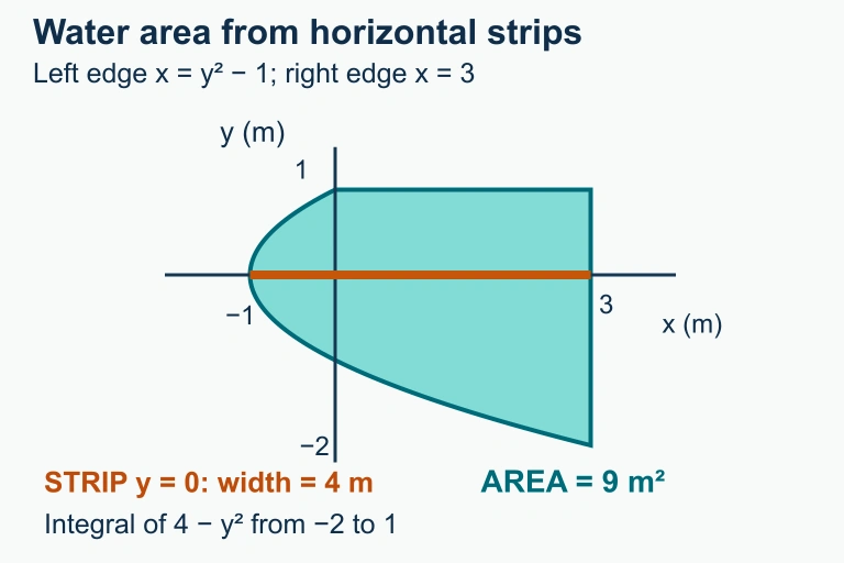Horizontal water strips span from x=y²−1 to x=3; filling through y=1 gives 9 m² of cross-sectional area. The water face is an explanatory cutaway, not an unsupported real water wall.

Question 5: CRITICAL THINKING

3 pts

Consider the region R enclosed by x = y³ − y and x = 0. (a) Find all y-values where the curves intersect. (b) Sketch the sign of the integrand y³ − y on each sub-interval and determine how many separate integrals are needed. (c) Set up and evaluate the integral(s) to find the total area of R.

Show answer

Part (a) — 1 point: Setting y³ − y = 0 gives y(y² − 1) = 0, so y(y − 1)(y + 1) = 0. The intersections are at y = −1, y = 0, and y = 1. Part (b) — 1 point: For −1 < y < 0, test y = −0.5: (−0.5)³ − (−0.5) = −0.125 + 0.5 = 0.375 > 0, so the curve x = y³ − y is to the RIGHT of x = 0. For 0 < y < 1, test y = 0.5: (0.5)³ − 0.5 = 0.125 − 0.5 = −0.375 < 0, so the curve is to the LEFT of x = 0. The roles of right and left switch at y = 0, so two separate integrals are needed. Part (c) — 1 point: A = ∫ from −1 to 0 [(y³ − y) − 0] dy + ∫ from 0 to 1 [0 − (y³ − y)] dy = ∫ from −1 to 0 (y³ − y) dy + ∫ from 0 to 1 (y − y³) dy. First integral: [y⁴/4 − y²/2] from −1 to 0 = 0 − (1/4 − 1/2) = 0 − (−1/4) = 1/4. Second integral: [y²/2 − y⁴/4] from 0 to 1 = (1/2 − 1/4) − 0 = 1/4. Total area = 1/4 + 1/4 = 1/2.

SUMMARY

Lesson Summary

Summary

To find the area between two curves expressed as functions of y, integrate (right function) − (left function) with respect to y over the interval defined by the y-coordinates of the intersection points. Each horizontal representative rectangle has infinitesimal height dy and length equal to the horizontal distance between the two curves at that y-value. The formula is A = ∫ from c to d [f(y) − g(y)] dy, where f(y) ≥ g(y) on [c, d].

Choose to integrate with respect to y when the curves are naturally expressed as x = f(y), when integrating with respect to x would require splitting the region into multiple integrals, or when boundary curves swap roles (top/bottom) across the x-interval. Always verify which curve is farther right by testing a sample y-value, and remember that if the right-left relationship changes within the interval, you must split the integral at the crossing y-value and use absolute value or swap functions accordingly.