Finding the Area Between Curves Expressed as Functions of x - AP Calculus AB

SECTION 1

Historical Context & Motivation

The problem of finding the area enclosed by curves is one of the oldest in mathematics, predating formal calculus by nearly two millennia. Ancient Greek geometers, most notably Archimedes, devised the method of exhaustion to approximate areas bounded by parabolas and other curves by inscribing sequences of polygons whose areas converged to the true value. This geometric technique foreshadowed the limit-based reasoning that would eventually give rise to integral calculus. For centuries, however, each new curve required its own bespoke geometric argument, and a general-purpose algorithm for computing enclosed areas remained elusive.

The breakthrough arrived in the seventeenth century when Isaac Newton and Gottfried Wilhelm Leibniz independently developed the Fundamental Theorem of Calculus, which linked the antiderivative to the definite integral and transformed area computation from a case-by-case geometric exercise into a systematic algebraic procedure. By expressing the area under a single curve as the definite integral of that function, and extending the idea to the difference of two functions, mathematicians gained the ability to compute the area of any region bounded by curves that could be written as functions of x.

~250 BCE • Archimedes and the Method of Exhaustion

Archimedes calculates the area under a parabolic arch by inscribing triangles, proving it equals ⁴⁄₃ the area of the inscribed triangle — an early triumph of limit-like reasoning.

1635 • Cavalieri's Principle of Indivisibles

Bonaventura Cavalieri introduces the concept of summing infinitely many thin slices to compute areas and volumes, laying algebraic groundwork for integration.

1666–1676 • Newton and Leibniz Develop Calculus

Working independently, Newton and Leibniz formalize the Fundamental Theorem of Calculus, unifying differentiation and integration and enabling systematic area computation.

1823 • Cauchy Formalizes the Definite Integral

Augustin-Louis Cauchy provides a rigorous epsilon-based definition of the definite integral, solidifying the theoretical foundation for area-between-curves problems.

1854 • Riemann's Integral Definition

Bernhard Riemann generalizes Cauchy's work with the Riemann sum, enabling integration of a broader class of functions and formalizing the area interpretation of the integral.

Today, finding the area between curves is one of the most fundamental applications of integration in the AP Calculus AB curriculum. The central question it addresses is straightforward yet powerful: given two functions f(x) and g(x) that bound a region over some interval, how do we compute the exact area of that enclosed region? Answering this question requires not only antiderivative skills but also a deep understanding of how definite integrals accumulate signed areas, and how subtracting one function from another isolates the region of interest.

SECTION 2

Core Principles & Definitions

Before diving into computations, it is essential to establish several foundational ideas that govern how we set up and evaluate area-between-curves integrals. Each principle below builds on your prior knowledge of definite integrals and extends it to the two-function setting that characterizes enclosed regions.

Top Minus Bottom

When f(x) ≥ g(x) on [a, b], the area between the curves equals ∫ from a to b of [f(x) − g(x)] dx. The integrand is always the upper function minus the lower function, ensuring the height of each infinitesimal rectangle is positive.

Intersection Points as Limits

The endpoints of integration are typically the x-coordinates where the two curves intersect, found by solving f(x) = g(x). These intersections define the horizontal extent of the enclosed region.

Splitting When Curves Cross

If the curves switch which is on top within the interval, you must split the integral at each crossing point. On each sub-interval, identify which function is greater and integrate accordingly, then sum the results.

Absolute Value Interpretation

Equivalently, the total area can be written as ∫ from a to b of |f(x) − g(x)| dx, which automatically accounts for sign changes. In practice, splitting into sub-intervals is more tractable for antiderivative computation.

Geometric Accumulation

The integral sums infinitely many vertical rectangular strips of width dx and height [f(x) − g(x)]. Each strip's area is its height times its infinitesimal width, and integration accumulates these strips across the interval.

✦

KEY TAKEAWAY

Think of the area between two curves like measuring the material between two fence lines running across a field. At each horizontal position x, you measure the vertical gap between the higher fence (the top curve) and the lower fence (the bottom curve). The total material — the area — is the continuous sum of all those vertical gaps, accumulated by the integral from one boundary post (the left intersection) to the other (the right intersection). If the fences cross, you must measure from whichever fence is higher at each position.

SECTION 3

Visual Explanation

The diagram below illustrates the fundamental geometric setup for computing the area between two curves expressed as functions of x. The shaded region represents the area we seek, bounded above by f(x) and below by g(x), with the limits of integration determined by the intersection points of the two curves.

The cyan curve represents f(x) (the upper function) and the violet curve represents g(x) (the lower function). The shaded gradient region between them is the area computed by the integral. The yellow dashed segment at a sample x-value shows the height f(x) − g(x) of one infinitesimal rectangular strip. The pink dots mark the intersection points at x = a and x = b, which serve as the limits of integration.

Observe how the vertical strip (shown in amber) represents the integrand f(x) − g(x) at a particular x-value. As x sweeps from a to b, the integral continuously sums these vertical strips, each of width dx. The shaded region is the accumulated total. This is the geometric heart of the method: the definite integral is a continuous summation device that adds up infinitely many infinitesimally thin rectangles to produce the exact enclosed area.

SECTION 4

Mathematical Framework

The mathematical machinery for computing the area between curves rests on the definite integral and the Fundamental Theorem of Calculus. We formalize the geometric intuition from the previous section into precise formulas that handle the standard case, the crossing-curves case, and the absolute-value shorthand.

BASIC AREA FORMULA

A = ∫ₐᵇ [f(x) − g(x)] dx, where f(x) ≥ g(x) on [a, b]

A = total enclosed area; f(x) = upper curve; g(x) = lower curve; a and b = x-coordinates of the left and right boundaries (often intersection points).

This formula applies directly when one function lies entirely above the other across the interval of integration. The requirement that f(x) ≥ g(x) ensures the integrand is non-negative, so the integral yields a positive area. If the problem does not specify which function is on top, you must determine the relative positions by testing a sample point in the interval or by graphing.

FINDING INTERSECTION POINTS

f(x) = g(x) → solve for x → x = a, x = b, …

Set the two functions equal and solve. The solutions give the x-values where the curves meet, which typically serve as the limits of integration.

SPLITTING AT CROSSING POINTS

A = ∫ₐᶜ [f(x) − g(x)] dx + ∫꜀ᵇ [g(x) − f(x)] dx

When the curves cross at x = c inside the interval [a, b], split the integral at c. On [a, c], if f(x) ≥ g(x), integrate f − g; on [c, b], if g(x) ≥ f(x), integrate g − f. Sum both positive quantities.

ABSOLUTE VALUE FORM

A = ∫ₐᵇ |f(x) − g(x)| dx

This compact form automatically handles sign changes. In practice, you must still remove the absolute value by splitting the interval at crossing points to evaluate the antiderivative.

⚠

AP Exam Tip

On the AP Calculus AB exam, a common error is to integrate f(x) − g(x) without verifying which function is on top across the entire interval, leading to a negative integrand on part of the domain and an undercount of the true area. Always check relative position by plugging in a test value from each sub-interval or by examining the graph provided.

SECTION 5

Handling Crossing Curves & Multi-Region Problems

Many area-between-curves problems on the AP exam involve functions that intersect more than once, creating multiple enclosed sub-regions. In these situations, the curves switch which is on top at each crossing point. This is the single most important complication to master, because failing to split the integral at crossing points is the leading source of sign errors in area computations. The diagram below illustrates a scenario where two curves cross inside the interval, producing two distinct shaded regions that must be integrated separately and then added.

The curves f(x) (cyan) and g(x) (violet) intersect at three points: x = a, x = c, and x = b. In Region I (left, cyan shading), f(x) lies above g(x), so we integrate f − g. In Region II (right, pink shading), g(x) lies above f(x), so we integrate g − f. The red dot at x = c marks the crossing point where the integrand changes sign.

The procedural algorithm for any area-between-curves problem can be summarized in a systematic sequence of steps.

Step 1 — Sketch or analyze the graph. Identify the two functions and determine where each one lies relative to the other. A graphing calculator (permitted on Part A of the free-response section) can help.
Step 2 — Find all intersection points. Solve f(x) = g(x) to determine the x-coordinates that serve as limits of integration.
Step 3 — Determine which function is on top. On each sub-interval between consecutive intersection points, test a sample x-value to see which function yields the larger y-value.
Step 4 — Set up and evaluate the integral(s). Write the integral as (top) − (bottom) on each sub-interval, evaluate each integral, and sum the results.

⚠

Common Pitfall

Some students attempt to evaluate a single integral ∫ₐᵇ [f(x) − g(x)] dx when the curves cross inside [a, b]. This produces a net signed area, which is smaller than the total geometric area because positive and negative contributions partially cancel. Always split at crossing points to avoid this error.

SECTION 6

Worked Example

Let us compute the exact area of the region enclosed by f(x) = x² and g(x) = x + 2. This is a classic AP-style problem that requires finding intersection points, identifying the upper and lower curves, setting up a single definite integral, and evaluating.

Area Between y = x² and y = x + 2

1
Step 1 — Find the intersection points

Set the functions equal: x² = x + 2. Rearrange to get x² − x − 2 = 0. Factor: (x − 2)(x + 1) = 0, giving x = −1 and x = 2. These are the limits of integration.

Intersection points: x = −1 and x = 2
2
Step 2 — Determine which function is on top

Test a sample point in (−1, 2). At x = 0: f(0) = 0² = 0 and g(0) = 0 + 2 = 2. Since g(0) > f(0), the line g(x) = x + 2 is above the parabola f(x) = x² throughout this interval.

Upper: g(x) = x + 2; Lower: f(x) = x²
3
Step 3 — Set up the integral

Area = ∫ from −1 to 2 of [(x + 2) − x²] dx = ∫ from −1 to 2 of (x + 2 − x²) dx.
4
Step 4 — Find the antiderivative

The antiderivative of (x + 2 − x²) is F(x) = x²/2 + 2x − x³/3.

F(x) = x²/2 + 2x − x³/3
5
Step 5 — Evaluate using the Fundamental Theorem

F(2) = (4/2) + 4 − (8/3) = 2 + 4 − 8/3 = 6 − 8/3 = 10/3. F(−1) = (1/2) + (−2) − (−1/3) = 1/2 − 2 + 1/3 = −7/6. Area = F(2) − F(−1) = 10/3 − (−7/6) = 10/3 + 7/6 = 20/6 + 7/6 = 27/6 = 9/2.

Area = 9/2 square units

💡

Verification Check

The result 9/2 = 4.5 is positive and has the correct units (square units). As a sanity check, the region fits inside a rectangle of width 3 and height roughly 4, giving an upper bound of 12 — and 4.5 is comfortably less than 12, confirming plausibility.

SECTION 7

Common Scenarios & Potential Pitfalls

Area-between-curves problems on the AP exam appear in several recognizable configurations. The table below categorizes the most common scenarios, identifies their distinguishing features, and highlights the specific pitfall associated with each. Developing fluency with these variations will prepare you for the range of problems you are likely to encounter.

Scenario	Setup & Features	Common Pitfall
One region, no crossing	f(x) ≥ g(x) on entire [a, b]. Single integral ∫ₐᵇ [f − g] dx.	Reversing the order (bottom − top) yields a negative value. Always verify sign.
Curves cross once inside [a, b]	Split into two integrals at the crossing point c. Sum both positive areas.	Using a single integral without splitting leads to partial cancellation of area.
Curves cross multiple times	Split at every crossing point. n crossings produce up to n + 1 sub-intervals.	Missing an intersection point omits an entire sub-region from the total.
Region bounded by a curve and the x-axis	g(x) = 0. Simplifies to ∫ₐᵇ \|f(x)\| dx, but still requires splitting if f changes sign.	Forgetting that ∫ₐᵇ f(x) dx gives signed area, not geometric area when f < 0.
Explicitly given limits (not intersections)	The problem provides specific values of a and b rather than requiring you to solve f = g.	Assuming the given limits are intersection points; curves may cross inside the interval.

Common area-between-curves configurations on the AP exam

✦

KEY TAKEAWAY

The area between curves is analogous to computing net pay in an engineering budget. If income f(x) exceeds expenses g(x), the surplus (area) is positive. If expenses exceed income on some sub-interval, you must account for that deficit separately — you cannot simply lump the whole period together without distinguishing the sign change, or the surpluses and deficits will mask each other. Splitting at crossing points is like closing the books at each sign-change date to get the true total absolute deviation from break-even.

SECTION 8

Connection to Advanced Topics

The technique of integrating with respect to x to find the area between curves is just one entry in a family of related methods. Understanding how this foundational approach connects to more advanced settings — particularly integrating with respect to y and computing volumes of revolution — helps you see the broader architectural pattern of applied integration and prepares you for both the AP exam and future coursework.

Feature	Area Between Curves (dx)	Area Between Curves (dy)
Integration variable	x (horizontal sweep)	y (vertical sweep)
Integrand structure	[top function] − [bottom function]	[right function] − [left function]
Rectangular strips	Vertical strips of width dx	Horizontal strips of width dy
Limits of integration	x-coordinates of boundary points	y-coordinates of boundary points
When to prefer	Curves easily expressed as y = f(x)	Curves more naturally expressed as x = h(y), or when dx setup requires multiple integrals

Comparison of dx vs. dy approaches for area between curves

Beyond area, the same "slice and accumulate" paradigm extends to volumes of solids of revolution (the disk, washer, and shell methods), where instead of summing rectangular strips, you sum circular disks or cylindrical shells. In Calculus BC and multivariable calculus, the principle extends further to double and triple integrals that compute areas and volumes in higher-dimensional settings. Mastering the dx area-between-curves technique provides the conceptual scaffolding for all of these extensions: identify the geometric element (strip, disk, shell), express its measure in terms of the integration variable, and sum over the appropriate interval.

ℹ

Looking Ahead

The washer method for volumes of revolution is a direct generalization of the area-between-curves formula. Where A = ∫ [f(x) − g(x)] dx sums vertical heights, the washer method sums π[f(x)² − g(x)²] dx — the area of each annular cross-section. Recognizing this structural parallel will make volumes feel like a natural extension rather than a new topic.

SECTION 9

Practice Problems

Question 1: CONCEPTUAL

When computing the area between two curves y = f(x) and y = g(x) on an interval [a, b], why is it necessary to determine which function is the upper curve before setting up the integral?

A. Because the Fundamental Theorem of Calculus only applies when the integrand is a polynomial.
B. Because integrating (lower − upper) produces a negative value, and area is a non-negative geometric quantity, so the integrand must be arranged to remain non-negative.
C. Because the antiderivative is undefined when the integrand is negative.
D. Because the upper curve always has a larger antiderivative, simplifying evaluation.
E. Because the intersection points change depending on which function is labeled f and which is labeled g.

Show answer (B)

The correct answer is B. Area is a non-negative quantity representing the size of a region, so the integrand must be non-negative throughout the interval. If we integrate (lower − upper), the integrand is negative, and the integral yields the negative of the area. Choice A is incorrect because the FTC applies to any continuous integrand, not just polynomials. Choice C is incorrect because antiderivatives exist for negative integrands — the sign of the function does not affect the existence of the antiderivative. Choice D is incorrect because having a larger antiderivative is neither guaranteed nor relevant to why order matters. Choice E is incorrect because intersection points are determined by where f(x) = g(x), which is symmetric — switching labels does not change the x-values.

Question 2: BASIC CALCULATION

Find the area of the region enclosed by y = x² and y = 4.

A. 16/3
B. 8/3
C. 32/3
D. 8
E. 64/3

Show answer (C)

The correct answer is C. First, find intersections: x² = 4 gives x = −2 and x = 2. On [−2, 2], the line y = 4 is above y = x², so the area is ∫ from −2 to 2 of (4 − x²) dx. The antiderivative is 4x − x³/3. Evaluating: [4(2) − 8/3] − [4(−2) − (−8/3)] = [8 − 8/3] − [−8 + 8/3] = (16/3) − (−16/3) = 32/3. Choice A (16/3) is half the correct answer, likely from integrating only from 0 to 2 without accounting for symmetry. Choice B (8/3) results from an algebraic error. Choice D (8) would be the area of the bounding rectangle from −2 to 2 with height 4, minus nothing — an incorrect setup. Choice E (64/3) doubles the correct answer, suggesting an error in evaluation.

Question 3: INTERMEDIATE

Find the total area of the regions enclosed between y = x³ − x and y = 0 on the interval [−1, 1].

A. 0
B. 1/4
C. 1/2
D. 1
E. 3/4

Show answer (C)

The correct answer is C. The function y = x³ − x factors as x(x − 1)(x + 1), so it crosses y = 0 at x = −1, 0, and 1. On [−1, 0], test x = −0.5: (−0.5)³ − (−0.5) = −0.125 + 0.5 = 0.375 > 0, so x³ − x ≥ 0 and the area is ∫₋₁⁰ (x³ − x) dx. On [0, 1], test x = 0.5: (0.5)³ − 0.5 = −0.375 < 0, so the x-axis is above and the area is ∫₀¹ −(x³ − x) dx = ∫₀¹ (x − x³) dx. Evaluating: ∫₋₁⁰ (x³ − x) dx = [x⁴/4 − x²/2] from −1 to 0 = 0 − (1/4 − 1/2) = 1/4. And ∫₀¹ (x − x³) dx = [x²/2 − x⁴/4] from 0 to 1 = 1/2 − 1/4 = 1/4. Total area = 1/4 + 1/4 = 1/2. Choice A (0) is the net signed integral, which cancels due to the odd symmetry of x³ − x — this gives signed area, not geometric area. Choice B (1/4) counts only one of the two regions. Choice D and E result from algebraic errors.

Question 4: APPLIED

3 pts

A civil engineer models the cross-section of a drainage channel. The bottom of the channel follows the curve y = x²/4 (in meters) and the water surface is at y = 3 (a horizontal line), where x is the horizontal distance from the center. Set up and evaluate the integral that gives the cross-sectional area of water in the channel.

Show answer

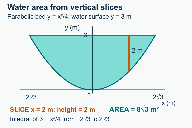Point 1 (1 pt): Find intersection points. Set x²/4 = 3, so x² = 12, giving x = −2√3 and x = 2√3. Point 2 (1 pt): Set up the integral correctly. The water surface y = 3 is above the channel bottom y = x²/4 on [−2√3, 2√3], so A = ∫ from −2√3 to 2√3 of (3 − x²/4) dx. Point 3 (1 pt): Evaluate the integral. Using symmetry: A = 2∫₀^{2√3} (3 − x²/4) dx = 2[3x − x³/12] from 0 to 2√3 = 2[3(2√3) − (2√3)³/12] = 2[6√3 − (24√3)/12] = 2[6√3 − 2√3] = 2(4√3) = 8√3 ≈ 13.86 square meters. Water above the parabolic bed y=x²/4 and below y=3, between x=−2√3 and x=2√3. A vertical slice at x=2 has height 2; total area is 8√3 m².

Water above the parabolic bed y=x²/4 and below y=3, between x=−2√3 and x=2√3. A vertical slice at x=2 has height 2; total area is 8√3 m².

The water cross-section lies between y=3 and the bed y=x²/4; vertical slice heights integrate to 8√3 m². The water face is an explanatory cutaway, not an unsupported real water wall.

Question 5: CRITICAL THINKING

4 pts

Let f and g be continuous functions on [0, 4] with the following properties: • f(x) ≥ g(x) on [0, 2] and g(x) ≥ f(x) on [2, 4]. • ∫₀⁴ f(x) dx = 10 and ∫₀⁴ g(x) dx = 8. • ∫₀² f(x) dx = 7 and ∫₀² g(x) dx = 3. (a) Find ∫₀² [f(x) − g(x)] dx. (b) Find ∫₂⁴ [g(x) − f(x)] dx. (c) Find the total area enclosed between the two curves on [0, 4]. (d) Explain why a student who computes ∫₀⁴ [f(x) − g(x)] dx obtains a value less than the true total area.

Show answer

Point 1 (1 pt) — Part (a): ∫₀² [f(x) − g(x)] dx = ∫₀² f(x) dx − ∫₀² g(x) dx = 7 − 3 = 4. Point 2 (1 pt) — Part (b): By the additive property of integrals, ∫₂⁴ f(x) dx = 10 − 7 = 3 and ∫₂⁴ g(x) dx = 8 − 3 = 5. Therefore ∫₂⁴ [g(x) − f(x)] dx = 5 − 3 = 2. Point 3 (1 pt) — Part (c): Total area = ∫₀² [f(x) − g(x)] dx + ∫₂⁴ [g(x) − f(x)] dx = 4 + 2 = 6. Point 4 (1 pt) — Part (d): Computing ∫₀⁴ [f(x) − g(x)] dx = 10 − 8 = 2. This is less than the true total area of 6 because on [2, 4], f(x) − g(x) < 0, so the integral counts the area of that region as negative. The positive contribution (4) and the negative contribution (−2) partially cancel, yielding the net signed area of 2 rather than the total geometric area of 6. To obtain the true area, you must split at the crossing point x = 2 and take the absolute value of each piece before summing.

SUMMARY

Lesson Summary

Summary

The area between two curves expressed as functions of x is computed by integrating the upper function minus the lower function with respect to x over the interval defined by the curves' intersection points. The formula A = ∫ₐᵇ [f(x) − g(x)] dx applies directly when f(x) ≥ g(x) throughout [a, b]. When the curves cross inside the interval, you must split the integral at each crossing point, compute the area of each sub-region with the correct (top − bottom) orientation, and sum the results.

The essential procedure is: (1) find intersection points by solving f(x) = g(x), (2) determine which function is on top on each sub-interval using a test point, (3) set up the integral(s) as (top − bottom), and (4) evaluate using antiderivatives and the Fundamental Theorem of Calculus. The absolute value form A = ∫ₐᵇ |f(x) − g(x)| dx provides a compact theoretical expression, but in practice the splitting approach is necessary for evaluation. This technique forms the foundation for more advanced applications including volumes of revolution and integration with respect to y.