Variations in Populations - AP Biology

SECTION 1

Historical Context & Motivation

The observation that individuals within a species are not identical has fascinated naturalists for centuries, yet the mechanisms generating and maintaining this phenotypic variation remained elusive until the fusion of Mendelian genetics with Darwinian selection in the early twentieth century. Charles Darwin recognized that heritable variation was the essential raw material for natural selection, but he could not explain how traits were inherited or how new variation arose. The rediscovery of Gregor Mendel's work on discrete hereditary factors, combined with advances in statistics and field ecology, ultimately forged the Modern Synthesis — the intellectual framework that unified genetics, paleontology, and population biology into a coherent theory of evolution. Understanding how variation originates, is distributed, and is acted upon by evolutionary forces remains a cornerstone of modern biology.

1859 • On the Origin of Species

Darwin publishes his theory of evolution by natural selection, emphasizing that heritable variation among individuals is essential for differential survival and reproduction.

1900 • Rediscovery of Mendel's Laws

De Vries, Correns, and von Tschermak independently rediscover Mendel's principles of segregation and independent assortment, providing a particulate basis for inheritance.

1908 • Hardy-Weinberg Principle

Hardy and Weinberg independently derive the equilibrium model showing that allele frequencies remain constant in an idealized population, establishing a null hypothesis for detecting evolutionary change.

1942 • The Modern Synthesis

Julian Huxley coins the term 'Modern Synthesis' to describe the integration of Darwinian selection with Mendelian genetics, population genetics (Fisher, Wright, Haldane), and systematics.

1968 • Neutral Theory of Molecular Evolution

Motoo Kimura proposes that much molecular variation is selectively neutral, maintained by mutation-drift balance rather than natural selection, broadening our view of population-level variation.

A central question emerged from this history: if natural selection favors the 'fittest' phenotype, why do populations retain so much genetic variation rather than converging on a single optimal genotype? Answering this question requires examining how mutation, recombination, gene flow, genetic drift, and selection interact to generate and maintain variation at both the genotypic and phenotypic levels.

SECTION 2

Core Principles of Population Variation

Variation in a population refers to the differences in traits — morphological, physiological, behavioral, and molecular — among individuals of the same species. For variation to drive evolution, it must be heritable, meaning it must have a genetic basis that can be transmitted from parent to offspring. Environmental factors can also produce phenotypic variation, but only genetically based differences contribute to evolutionary change across generations.

Mutation

Random changes in DNA sequence — point mutations, insertions, deletions, and chromosomal rearrangements — are the ultimate source of all new alleles. Mutations are rare per locus per generation but accumulate over time and across the genome.

Sexual Reproduction & Recombination

Crossing over during meiosis and the independent assortment of chromosomes generate novel allele combinations each generation. Sexual reproduction does not create new alleles but dramatically increases genotypic diversity.

Gene Flow

The migration of alleles between populations introduces new genetic variants and tends to homogenize allele frequencies among populations, counteracting divergence caused by drift or local selection.

Genetic Drift

Random fluctuations in allele frequency are most pronounced in small populations. Drift can reduce variation by fixing or eliminating alleles regardless of their adaptive value, as seen in bottleneck and founder effects.

Natural Selection

Differential survival and reproduction based on phenotype can increase, decrease, or maintain variation depending on the mode of selection — directional, stabilizing, or disruptive.

✦

KEY TAKEAWAY

Think of a population's gene pool as a deck of cards. Mutation adds new cards to the deck, recombination shuffles existing cards into new hands, gene flow trades cards with another player's deck, drift randomly removes cards from the game, and selection decides which hands are played. The interplay of these forces determines how much variation the deck retains over time.

SECTION 3

Visualizing the Sources of Variation

The central gene pool receives new alleles via mutation and novel combinations via recombination. Gene flow exchanges alleles between populations, while genetic drift stochastically removes them. Natural selection (dashed arrow) acts as a filter on the variation already present.

The diagram above illustrates the relationship between the forces that generate, redistribute, and deplete genetic variation. Mutation is unique in that it is the only mechanism capable of producing new alleles; all other processes act upon pre-existing genetic material. Recombination amplifies the combinatorial possibilities of those alleles through crossing over and independent assortment during meiosis, which is why sexually reproducing species typically harbor far more phenotypic diversity than asexual lineages. Gene flow can either increase or decrease local variation depending on whether incoming alleles are novel or common, while genetic drift tends to erode variation — an effect inversely proportional to population size. Natural selection may increase, decrease, or stabilize variation depending on its mode, a topic we will explore in detail in Section 5.

SECTION 4

Mathematical Framework: Hardy-Weinberg & Measuring Variation

Population genetics provides a quantitative framework for measuring variation and detecting evolutionary change. The Hardy-Weinberg equilibrium serves as the null model: it predicts allele and genotype frequencies in a population where no evolution is occurring. Any statistically significant deviation from Hardy-Weinberg expectations signals that one or more evolutionary forces — mutation, selection, drift, gene flow, or nonrandom mating — are altering the distribution of variation.

HARDY-WEINBERG ALLELE FREQUENCY

p + q = 1

For a locus with two alleles: p = frequency of the dominant allele; q = frequency of the recessive allele.

HARDY-WEINBERG GENOTYPE FREQUENCY

p² + 2pq + q² = 1

p² = frequency of homozygous dominant; 2pq = frequency of heterozygotes; q² = frequency of homozygous recessive.

The five conditions required for Hardy-Weinberg equilibrium — no mutation, random mating, no selection, no genetic drift (infinite population size), and no gene flow — are never perfectly met in nature. Their violation is precisely what makes the model useful: by comparing observed genotype frequencies to Hardy-Weinberg predictions, biologists can infer which evolutionary forces are at work and quantify the extent of their influence.

HETEROZYGOSITY (H)

H = 1 − Σ pᵢ²

Expected heterozygosity, where pᵢ is the frequency of the i-th allele at a locus. Higher H indicates greater genetic variation. When H = 0, the population is fixed for a single allele.

💡

AP EXAM TIP

The AP Biology exam frequently asks you to calculate allele or genotype frequencies using the Hardy-Weinberg equations. The most common entry point is the frequency of the homozygous recessive phenotype (q²), from which you can derive q, then p = 1 − q, and finally 2pq for carrier frequency. Practice working backwards from phenotype data to allele frequencies.

SECTION 5

Modes of Natural Selection and Their Effects on Variation

Natural selection does not always reduce variation. The three classical modes of selection — directional, stabilizing, and disruptive — have qualitatively different effects on the distribution of phenotypic variation within a population. These modes are best understood by visualizing how each shifts or reshapes the bell-shaped normal distribution of a continuous trait.

The three modes of selection reshape phenotypic distributions differently. Directional selection shifts the mean toward one extreme, stabilizing selection narrows the distribution around the existing mean, and disruptive selection creates a bimodal distribution by favoring both extremes. Dashed curves represent the original distribution before selection.

Additional mechanisms that maintain variation include heterozygote advantage (balancing selection), where the heterozygous genotype has higher fitness than either homozygote — the classic example being sickle-cell trait and malaria resistance. Frequency-dependent selection maintains multiple alleles because the fitness of a phenotype depends on its relative abundance in the population; rare phenotypes often have an advantage (negative frequency dependence), preventing any single allele from reaching fixation. Diploidy itself preserves variation by sheltering recessive alleles from selection when they are present in heterozygotes.

SECTION 6

Worked Example: Hardy-Weinberg Analysis of Variation

A population of 500 wildflowers exhibits two color phenotypes controlled by a single gene with two alleles. Red (R) is dominant to white (r). A field survey counts 80 white-flowered individuals. Determine the allele frequencies and the expected number of heterozygous (carrier) plants under Hardy-Weinberg assumptions.

Hardy-Weinberg Allele & Genotype Frequency Calculation

1
Step 1 — Determine q² from phenotype data

White-flowered plants are homozygous recessive (rr). Their frequency is q² = 80 / 500 = 0.16.

q² = 0.16
2
Step 2 — Solve for q

Take the square root of q²: q = √0.16 = 0.4. This is the frequency of the recessive allele (r) in the population.

q = 0.4
3
Step 3 — Solve for p

Since p + q = 1, we have p = 1 − 0.4 = 0.6. This is the frequency of the dominant allele (R).

p = 0.6
4
Step 4 — Calculate heterozygote frequency (2pq)

The frequency of heterozygous individuals is 2pq = 2 × 0.6 × 0.4 = 0.48. This means 48% of the population is expected to be carriers (Rr).

2pq = 0.48
5
Step 5 — Convert to expected number of individuals

In a population of 500: expected heterozygotes = 0.48 × 500 = 240 plants. We can verify the full distribution: p² × 500 = 0.36 × 500 = 180 (RR); 2pq × 500 = 240 (Rr); q² × 500 = 80 (rr). Total = 180 + 240 + 80 = 500. ✓

Expected heterozygotes = 240 plants

ℹ

NOTE

Notice that nearly half the population (48%) carries the recessive allele in heterozygous form, even though only 16% display the recessive phenotype. This demonstrates how diploidy preserves hidden variation — a key concept tested on the AP exam.

SECTION 7

Comparing Evolutionary Forces & Their Effects on Variation

Evolutionary Force	Effect on Variation	Population Size Dependency
Mutation	Introduces new alleles; always increases variation (slowly)	Independent — rate per gene per generation is constant
Recombination	Creates new allele combinations; increases genotypic diversity	Greater effect in large, genetically diverse populations
Gene Flow	Increases local variation; homogenizes variation among populations	Most impactful when populations differ in allele frequencies
Genetic Drift	Reduces variation by randomly fixing/eliminating alleles	Strongest in small populations (bottleneck/founder effects)
Natural Selection	Depends on mode: directional/stabilizing decrease; disruptive/balancing increase	More effective in large populations where drift is minimal

Summary of evolutionary forces and their effects on genetic variation within and among populations

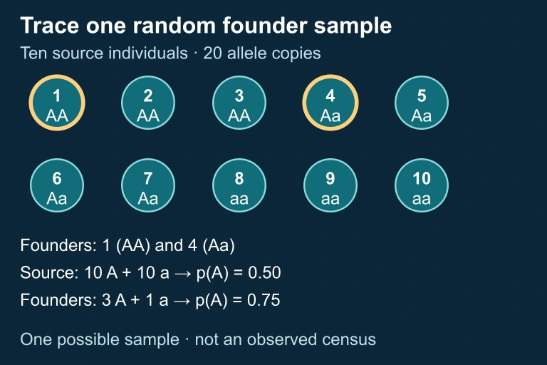Ten genotypes and founder sample

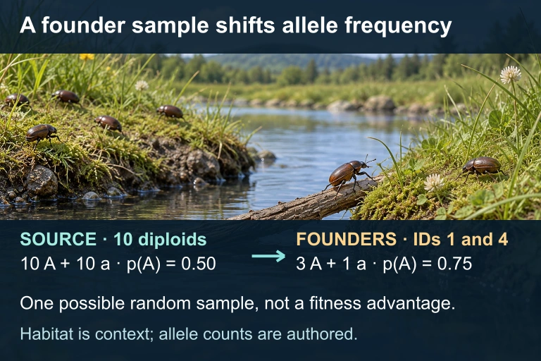A beetle habitat accompanies a hypothetical source-to-founder comparison. An authored companion lists ten genotypes and highlights founders 1 AA and 4 Aa. A founder event can change allele frequencies through sampling without a fitness advantage. In this synthetic example, 10 source diploids carry 10 A and 10 a copies; founders 1 and 4 carry 3 A and 1 a. The habitat image is contextual, not a measured sample.

✦

KEY TAKEAWAY

Variation in a population reflects a dynamic equilibrium — much like the water level in a bathtub with both the faucet (mutation, gene flow, disruptive selection) and the drain (drift, directional selection, stabilizing selection) running simultaneously. The 'water level' of genetic variation at any given moment depends on the relative rates of these opposing processes. In population genetics, this balance determines a population's evolutionary potential — its capacity to adapt to future environmental changes.

SECTION 8

Connections to Advanced Evolutionary Theory

The study of population-level variation connects directly to several advanced topics that extend beyond the AP Biology curriculum but provide important conceptual depth. Understanding how variation is structured within and among populations is foundational to quantitative genetics, phylogeography, and conservation genetics.

AP Biology Concept	Advanced Extension
Hardy-Weinberg equilibrium as null model	F-statistics (Fₛₜ) quantify population subdivision and divergence among subpopulations
Genetic drift in small populations	Effective population size (Nₑ) models predict rate of heterozygosity loss over generations
Heterozygote advantage (sickle-cell)	Multi-locus models of balancing selection, including overdominance and antagonistic pleiotropy
Phenotypic variation in continuous traits	Genome-wide association studies (GWAS) identify loci contributing to polygenic trait variation
Mutations as source of variation	Neutral theory and nearly neutral theory model mutation-drift equilibria at the molecular level

How AP-level concepts connect to advanced topics in population and evolutionary genetics

In conservation biology, maintaining genetic variation within endangered populations is a primary management goal. Small, isolated populations are susceptible to inbreeding depression — the reduction in fitness caused by increased homozygosity, which exposes deleterious recessive alleles. Strategies such as genetic rescue (introducing individuals from genetically distinct populations to restore heterozygosity) directly apply the principles of gene flow and variation maintenance covered in this lesson. The Florida panther recovery program, in which Texas pumas were introduced to the inbred Florida population, is a celebrated example of applied population genetics.

SECTION 9

Practice Problems

Question 1: CONCEPTUAL

Which of the following is the ultimate source of new genetic variation in a population?

A. Natural selection
B. Genetic recombination
C. Mutation
D. Genetic drift

Show answer (C)

C is correct. Mutation is the only process that generates entirely new alleles by altering DNA sequence. Natural selection (A) acts on existing variation but does not create new alleles. Genetic recombination (B) shuffles existing alleles into new combinations during meiosis but does not produce novel alleles. Genetic drift (D) is a random change in allele frequency that reduces variation rather than creating it.

Question 2: BASIC CALCULATION

In a population of 1,000 individuals, 90 display the homozygous recessive phenotype for a trait controlled by a single gene with two alleles. Assuming Hardy-Weinberg equilibrium, what is the expected frequency of heterozygous carriers?

A. 0.18
B. 0.42
C. 0.49
D. 0.30

Show answer (B)

B is correct. The frequency of the homozygous recessive phenotype is q² = 90/1000 = 0.09, so q = √0.09 = 0.3 and p = 1 − 0.3 = 0.7. The heterozygote frequency is 2pq = 2 × 0.7 × 0.3 = 0.42. Choice A (0.18) represents q² × 2 rather than 2pq. Choice C (0.49) equals p² and represents the homozygous dominant frequency. Choice D (0.30) is simply q, the recessive allele frequency, not the heterozygote frequency.

Question 3: INTERMEDIATE

A researcher observes that the mean body size of a lizard population has not changed over 20 generations, but the variance in body size has decreased significantly. Which mode of selection best explains this observation?

A. Directional selection
B. Disruptive selection
C. Stabilizing selection
D. Frequency-dependent selection

Show answer (C)

C is correct. Stabilizing selection favors intermediate phenotypes and selects against extremes, which reduces phenotypic variance while keeping the mean constant. Directional selection (A) would shift the mean toward one extreme. Disruptive selection (B) would increase variance by favoring both extremes. Frequency-dependent selection (D) maintains variation by giving rare phenotypes an advantage, which would not predictably decrease variance in this manner.

Question 4: APPLIED

4 pts

A conservation biologist is concerned that a population of bighorn sheep isolated on a mountain range has experienced significant loss of genetic variation due to a recent bottleneck event. Design an experiment to (a) measure the current level of genetic variation in the population, (b) compare it to a reference population that did not experience a bottleneck, and (c) propose a management intervention to restore variation. Include a null hypothesis and identify the independent and dependent variables.

Show answer

Point 1 (Null Hypothesis & Variables): H₀: There is no significant difference in expected heterozygosity (H) between the bottlenecked mountain population and the non-bottlenecked reference population. Independent variable: bottleneck history (bottlenecked vs. non-bottlenecked population). Dependent variable: expected heterozygosity (H) calculated from microsatellite or SNP genotype data. Point 2 (Measuring Variation): Collect tissue samples (e.g., ear notch biopsies) from ≥30 individuals in both the bottlenecked population and a large, stable reference population. Genotype individuals at 10–15 neutral microsatellite loci. Calculate expected heterozygosity (H = 1 − Σpᵢ²), observed heterozygosity, number of alleles per locus, and allelic richness for both populations. Point 3 (Statistical Comparison): Compare heterozygosity and allelic richness between the two populations using a Wilcoxon signed-rank test or permutation test across loci. Test for Hardy-Weinberg equilibrium deviations to detect inbreeding (excess homozygosity). If the bottlenecked population shows significantly lower heterozygosity, reject H₀. Point 4 (Management Intervention): Propose genetic rescue by translocating a small number (5–10) of unrelated individuals from the reference population into the bottlenecked population. This gene flow introduces new alleles, increases heterozygosity, and can alleviate inbreeding depression. Monitor heterozygosity and fitness metrics (survival, reproductive success) over subsequent generations to evaluate effectiveness.

Question 5: CRITICAL THINKING

4 pts

A researcher studying a population of beetles sampled allele frequencies at a coat-color locus over five years. The population size is approximately 50 individuals. The data are as follows: Year 1: p = 0.50, q = 0.50 Year 2: p = 0.54, q = 0.46 Year 3: p = 0.48, q = 0.52 Year 4: p = 0.60, q = 0.40 Year 5: p = 0.62, q = 0.38 (a) Describe the pattern observed in the allele frequency data. (b) Explain which evolutionary mechanism is most likely responsible and justify your reasoning. (c) Predict what would happen to allele frequencies if the population size increased to 10,000 and no selection was occurring. (d) Explain how this pattern affects genetic variation in the population over time.

Show answer

Point 1 — Pattern Description: The allele frequencies fluctuate unpredictably between years (e.g., p increases from 0.50 to 0.54, then decreases to 0.48, then increases to 0.60 and 0.62). There is a general trend of the p allele increasing, but the changes are erratic rather than consistently directional. Point 2 — Mechanism Identification: Genetic drift is the most likely mechanism. The small population size (N = 50) makes random sampling error during reproduction a powerful force. The erratic, non-directional fluctuations in allele frequency are characteristic of drift rather than selection, which would produce a more consistent directional trend. If selection were operating, we would expect p to move monotonically in one direction rather than oscillating. Point 3 — Prediction with Large Population: If the population size increased to 10,000 with no selection, allele frequencies would remain approximately stable generation to generation, as predicted by Hardy-Weinberg equilibrium. Random drift is inversely proportional to population size, so the stochastic fluctuations observed in the small population would be negligible in a population of 10,000. Point 4 — Effect on Variation: Over time, genetic drift in this small population will reduce genetic variation. One allele will eventually become fixed (frequency = 1.0) while the other is lost (frequency = 0.0). The rate of heterozygosity loss per generation is approximately 1/(2N) = 1/100 = 1% per generation. This progressive loss of variation decreases the population's adaptive potential and may increase susceptibility to environmental changes.

SUMMARY

Variations in Populations — Summary

Summary

Genetic variation within populations is the essential raw material for evolution by natural selection. Mutation is the ultimate source of all new alleles, while sexual reproduction and recombination generate novel allele combinations each generation. Gene flow introduces alleles from other populations, and genetic drift stochastically removes alleles — especially in small populations experiencing bottleneck or founder effects.

The Hardy-Weinberg equilibrium (p + q = 1; p² + 2pq + q² = 1) provides the null model for detecting departures caused by evolutionary forces. The three modes of selection reshape phenotypic distributions differently: directional selection shifts the mean, stabilizing selection narrows the distribution, and disruptive selection creates bimodal peaks. Mechanisms like heterozygote advantage, frequency-dependent selection, and diploidy help populations maintain the variation that fuels ongoing adaptation.