Population Genetics - AP Biology

SECTION 1

Historical Context & Motivation

Darwin's theory of evolution by natural selection, published in 1859, offered a compelling mechanism for adaptive change, yet it lacked a coherent model of inheritance. Blending inheritance—the prevailing idea that parental traits mix like paints—would quickly erode the very variation that selection requires. Gregor Mendel's work on discrete hereditary factors went largely unnoticed until its rediscovery in 1900, setting the stage for a synthesis between genetics and evolution. The challenge was mathematical: how could particulate inheritance be reconciled with the gradual, population-level changes Darwin described? Resolving this question gave rise to the field of population genetics, which treats evolution not as a change in individuals but as a shift in allele frequencies within breeding populations over time.

1866 • Mendel's Laws of Inheritance

Gregor Mendel publishes his experiments on pea plants, establishing the principles of segregation and independent assortment—though the work remains obscure for decades.

1908 • Hardy–Weinberg Principle

G. H. Hardy and Wilhelm Weinberg independently demonstrate that allele frequencies remain constant in the absence of evolutionary forces, providing a null model for population genetics.

1930–1932 • The Modern Synthesis Begins

R. A. Fisher, J. B. S. Haldane, and Sewall Wright formalize the mathematics of natural selection, genetic drift, and gene flow, unifying Mendelian genetics with Darwinian evolution.

1966 • Lewontin & Hubby — Protein Electrophoresis

Electrophoretic surveys reveal far more genetic variation in natural populations than predicted, stimulating the neutralist–selectionist debate and modern molecular population genetics.

2000s–present • Genomic Population Genetics

Whole-genome sequencing enables genome-wide scans for selection signatures, refined estimates of effective population size, and detailed reconstruction of demographic history.

The central question that population genetics answers is deceptively simple: What causes allele frequencies to change—or remain stable—from one generation to the next? Every evolutionary mechanism—natural selection, genetic drift, mutation, migration, and nonrandom mating—can be understood as a departure from the equilibrium predicted by the Hardy–Weinberg model. By quantifying these departures, biologists gain predictive power over the trajectory of populations, the maintenance of genetic diversity, and the molecular signatures left by adaptation.

SECTION 2

Core Principles of Population Genetics

Population genetics operates at the interface of genetics and evolutionary biology, analyzing how the genetic composition of populations shifts over time. Rather than tracking a single organism's genotype, the field focuses on allele frequencies and genotype frequencies across an entire breeding population, sometimes called a gene pool. The following foundational ideas underpin virtually every analysis in the discipline.

Allele Frequency

The proportion of a specific allele among all copies of that gene in a population. For a diploid locus with two alleles, frequencies are denoted p and q, where p + q = 1.

Hardy–Weinberg Equilibrium

A mathematical null model stating that allele and genotype frequencies remain constant across generations in the absence of mutation, selection, drift, migration, and nonrandom mating.

Genetic Drift

Random fluctuations in allele frequency due to finite population size. Drift has the greatest effect in small populations and can lead to fixation or loss of alleles independent of their fitness effects.

Gene Flow (Migration)

The movement of alleles between populations through migration of individuals or gametes. Gene flow tends to homogenize allele frequencies across populations and counteracts local adaptation.

Natural Selection at the Population Level

Differential survival and reproduction among genotypes alters allele frequencies directionally. Selection is the only evolutionary force that consistently produces adaptation.

✦

KEY TAKEAWAY

Think of Hardy–Weinberg equilibrium like a perfectly balanced chemical reaction at equilibrium: the system remains unchanged unless an external force perturbs it. In population genetics, the 'external forces' are the five agents of evolutionary change—mutation, selection, drift, gene flow, and nonrandom mating. Identifying which agent is acting, and how strongly, is the central challenge of the field. The Hardy–Weinberg model gives you the baseline expectation so you can detect departures and diagnose their causes.

SECTION 3

Visualizing Allele Frequency & Hardy–Weinberg Equilibrium

The diagram below illustrates how a population's allele frequencies (p and q) translate into the three possible genotype frequencies under Hardy–Weinberg equilibrium. The parabolic curve shows how the frequency of heterozygotes (2pq) is maximized when p = q = 0.5, and how homozygote frequencies change as one allele becomes dominant in the population.

As the frequency of allele A (p) increases from 0 to 1, the frequency of AA homozygotes (purple curve, p²) rises while aa homozygotes (pink curve, q²) fall. Heterozygote frequency (cyan curve, 2pq) peaks at 0.50 when p = q = 0.5. All three curves sum to 1.0 at every value of p.

Several features of this graph are worth internalizing. First, heterozygotes are the most common genotype whenever p is between roughly 0.33 and 0.67—this means that in many real populations, carriers of a recessive allele far outnumber homozygous affected individuals. Second, a rare recessive allele (e.g., q = 0.01) produces very few homozygous recessive individuals (q² = 0.0001, or 1 in 10,000), yet the carrier frequency is about 2 × 0.01 × 0.99 ≈ 0.02, or 1 in 50. This discrepancy explains why selection against recessive phenotypes is slow: most copies of the allele hide in heterozygotes.

SECTION 4

Mathematical Framework

The Hardy–Weinberg equations provide the quantitative backbone of population genetics. For a single autosomal locus with two alleles (A and a), let p represent the frequency of allele A and q represent the frequency of allele a. Because there are only two alleles, these frequencies must sum to unity.

ALLELE FREQUENCY IDENTITY

p + q = 1

Where p = frequency of the dominant allele (A) and q = frequency of the recessive allele (a). This relationship holds for any two-allele system.

HARDY–WEINBERG GENOTYPE FREQUENCIES

p² + 2pq + q² = 1

p² = frequency of AA homozygotes; 2pq = frequency of Aa heterozygotes; q² = frequency of aa homozygotes. This equation is derived by expanding (p + q)², reflecting the random union of gametes under HW assumptions.

The Hardy–Weinberg model rests on five assumptions: (1) no mutation introducing new alleles, (2) random mating with respect to the locus in question, (3) no natural selection favoring any genotype, (4) infinitely large population size (no genetic drift), and (5) no gene flow into or out of the population. When any of these conditions is violated, allele frequencies can change across generations—in other words, evolution occurs.

CALCULATING ALLELE FREQUENCY FROM GENOTYPE DATA

p = (2 × count of AA + count of Aa) / (2 × total individuals)

Each individual carries two alleles. AA individuals contribute 2 copies of A; heterozygotes contribute 1. Dividing by twice the population size (total allele count) gives the frequency of A.

SELECTION COEFFICIENT AND FITNESS

w = 1 − s

Where w = relative fitness of a genotype and s = selection coefficient (the proportional reduction in fitness compared to the most-fit genotype, which has w = 1). A lethal genotype has s = 1 (w = 0); a neutral allele has s = 0 (w = 1).

💡

AP EXAM TIP

On the AP Biology exam, the most common entry point into a Hardy–Weinberg problem is a stated frequency of the homozygous recessive phenotype. Because q² equals the frequency of the recessive phenotype, you take the square root to find q, then compute p = 1 − q, and finally derive p², 2pq, and q². Be ready to compare observed genotype frequencies to expected HW values and explain which evolutionary force likely accounts for any discrepancy.

SECTION 5

Five Agents of Evolutionary Change

Each violation of a Hardy–Weinberg assumption corresponds to an evolutionary mechanism. Understanding how these five forces differ in their directionality, magnitude, and dependence on population size is essential for AP Biology. The diagram below provides a conceptual overview of how each force shifts allele frequencies away from equilibrium.

Each of the five evolutionary forces feeds into the gene pool and perturbs allele or genotype frequencies. Nonrandom mating changes genotype frequencies without altering allele frequencies directly, while the other four forces change allele frequencies themselves.

Evolutionary Force	Direction	Effect on Variation	Population Size Dependence
Mutation	Random; introduces novel alleles	Increases variation	Weak per generation; rate independent of N
Natural Selection	Directional, stabilizing, or disruptive	Can increase or decrease variation	More effective in large N (overwhelms drift)
Genetic Drift	Random; unpredictable direction	Decreases variation (fixation/loss)	Strongest in small N
Gene Flow	Toward homogenization between populations	Increases within-pop variation; decreases between-pop variation	Depends on migration rate, not N per se
Nonrandom Mating	Alters genotype frequencies, not allele frequencies directly	Increases homozygosity (inbreeding); may increase variation in assortative	Independent of N

Comparison of the five evolutionary forces and their properties

Two special cases of genetic drift merit attention for the AP exam. A bottleneck effect occurs when a population undergoes a drastic reduction in size—due to a natural disaster, disease, or overhunting—so that the surviving gene pool is a small, potentially unrepresentative sample of the original. A founder effect arises when a small group of individuals colonizes a new habitat, carrying with them only a fraction of the genetic diversity of the source population. In both scenarios, rare alleles may be lost or dramatically overrepresented, and the resulting population may differ substantially from Hardy–Weinberg expectations.

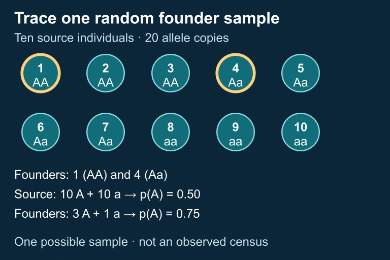Ten genotypes and founder sample

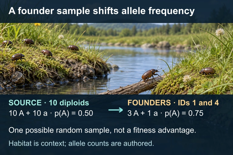A beetle habitat accompanies a hypothetical source-to-founder comparison. An authored companion lists ten genotypes and highlights founders 1 AA and 4 Aa. A founder event can change allele frequencies through sampling without a fitness advantage. In this synthetic example, 10 source diploids carry 10 A and 10 a copies; founders 1 and 4 carry 3 A and 1 a. The habitat image is contextual, not a measured sample.

SECTION 6

Worked Example: Applying Hardy–Weinberg

Consider a population of 500 wildflowers exhibiting flower color determined by a single locus with two alleles: C (red, dominant) and c (white, recessive). A survey reveals that 80 plants have white flowers. Determine allele and genotype frequencies assuming Hardy–Weinberg equilibrium, then calculate the expected number of heterozygous plants.

Hardy–Weinberg Calculation: Wildflower Population

1
Step 1 — Identify the Known Quantity

White flowers are the recessive phenotype, so white plants have genotype cc. The frequency of the homozygous recessive phenotype is q² = 80 / 500 = 0.16.

q² = 0.16
2
Step 2 — Find q

Take the square root of q² to obtain the frequency of the recessive allele c: q = √0.16 = 0.4.

q = 0.4
3
Step 3 — Find p

Since p + q = 1, the frequency of the dominant allele C is p = 1 − 0.4 = 0.6.

p = 0.6
4
Step 4 — Calculate Genotype Frequencies

Apply the Hardy–Weinberg equation: p² = (0.6)² = 0.36 (frequency of CC); 2pq = 2 × 0.6 × 0.4 = 0.48 (frequency of Cc); q² = 0.16 (frequency of cc). Verify: 0.36 + 0.48 + 0.16 = 1.00 ✓.

p² = 0.36, 2pq = 0.48, q² = 0.16
5
Step 5 — Expected Number of Heterozygotes

Multiply the heterozygote frequency by the total population: 0.48 × 500 = 240 plants are expected to be heterozygous (Cc). Note that these plants display the dominant red phenotype, yet they each carry one copy of the recessive white allele—making them carriers.

Expected heterozygotes = 240 plants

ℹ

WHY THIS MATTERS

Notice that 80 plants show the recessive phenotype, but 240 carry the recessive allele in heterozygous form. This means three times as many plants carry the allele as actually express it—a critical insight for understanding why recessive conditions persist in populations and why selection against recessive phenotypes is slow.

SECTION 7

Strengths and Limitations of the Hardy–Weinberg Model

Like any model in science, Hardy–Weinberg equilibrium is both powerful and limited. Its primary value lies not in describing real populations—few truly meet all five assumptions—but in serving as a rigorous null hypothesis against which observed data can be tested. When genotype frequencies deviate significantly from HW expectations, the model directs investigators toward identifying which evolutionary force is responsible.

Strengths	Limitations
Provides a clear null model: any deviation implies evolution is occurring	Assumes only two alleles at one locus; real traits are often polygenic
Allows estimation of carrier frequencies from phenotypic data (useful in medical genetics)	Assumes infinite population size; all real populations are finite and subject to drift
Mathematically simple yet widely applicable across diploid organisms	Cannot distinguish among multiple simultaneous violations (e.g., selection + drift)
Genotype frequencies reach equilibrium after just one generation of random mating	Assumes non-overlapping generations and no age structure

Strengths and limitations of the Hardy–Weinberg equilibrium model

✦

KEY TAKEAWAY

Hardy–Weinberg equilibrium functions much like a control group in an experiment. Just as a control tells you what would happen without the experimental treatment, the HW model tells you what allele and genotype frequencies would look like without any evolutionary force acting. Departures from HW are the 'signal'—your job on the AP exam is to diagnose which force (or forces) produced that signal.

SECTION 8

Connections to Advanced Evolutionary Theory

Population genetics provides the theoretical foundation for several advanced topics you may encounter in college-level biology or on the AP exam's more challenging free-response questions. Understanding how basic HW analysis connects to these deeper frameworks strengthens your ability to interpret complex scenarios involving multiple evolutionary forces acting simultaneously.

Basic Population Genetics (AP Level)	Advanced Extension
Two-allele HW model at one locus	Multi-allele and multi-locus models; linkage disequilibrium between loci
Directional selection changes allele frequencies	Balancing selection (heterozygote advantage, frequency-dependent selection) maintains polymorphism
Genetic drift as random allele frequency change	Effective population size (Nₑ); coalescent theory tracing alleles backward in time
Gene flow homogenizes populations	Landscape genetics; FST statistics quantifying population differentiation
Fitness (w) and selection coefficient (s)	Quantitative genetics: heritability (h²), response to selection (R = h² × S), polygenic adaptation

Bridging AP-level population genetics to advanced evolutionary theory

One particularly important extension is heterozygote advantage (also called overdominance), in which heterozygous individuals have higher fitness than either homozygote. The classic example is sickle-cell anemia in regions with endemic malaria: individuals heterozygous for the hemoglobin S allele (HbA/HbS) gain protection from malaria without developing sickle-cell disease. This form of balancing selection maintains both alleles in the population at a stable equilibrium frequency—a phenomenon that straightforward directional selection would not predict. On the AP exam, recognizing when a polymorphism is maintained by heterozygote advantage rather than being driven to fixation can distinguish a strong from a weak response.

📝

LOOKING AHEAD

At the college level, population genetics merges with genomics to answer questions about human migration patterns, conservation of endangered species, and the evolution of antibiotic resistance. The same Hardy–Weinberg framework you learn here is the starting point for all of these investigations—only the complexity of the models increases.

SECTION 9

Practice Problems

Question 1: CONCEPTUAL

Which of the following is a necessary condition for a population to remain in Hardy–Weinberg equilibrium?

A. Natural selection must favor the heterozygous genotype.
B. Individuals must mate randomly with respect to the locus in question.
C. The population must have undergone a recent bottleneck to establish initial frequencies.
D. Mutation must continually introduce new alleles to maintain genetic variation.

Show answer (B)

B is correct. Random mating is one of the five assumptions of Hardy–Weinberg equilibrium; nonrandom mating (such as assortative mating or inbreeding) shifts genotype frequencies away from HW expectations. A is incorrect because any form of natural selection—including heterozygote advantage—violates the no-selection assumption. C is incorrect because a bottleneck introduces genetic drift, which itself violates the infinite population size assumption. D is incorrect because the HW model requires no mutation; mutation introduces new alleles and changes allele frequencies.

Question 2: BASIC CALCULATION

In a population of 1,000 individuals, 90 express the recessive phenotype for a trait controlled by a single autosomal locus with two alleles. Assuming Hardy–Weinberg equilibrium, what is the expected frequency of carriers (heterozygotes)?

A. 0.09
B. 0.42
C. 0.30
D. 0.49

Show answer (B)

B is correct. The frequency of the homozygous recessive phenotype is q² = 90/1000 = 0.09. Taking the square root, q = 0.3, so p = 1 − 0.3 = 0.7. The heterozygote frequency is 2pq = 2 × 0.7 × 0.3 = 0.42. A (0.09) is q², the homozygous recessive frequency, not the heterozygote frequency. C (0.30) is the value of q itself, not 2pq. D (0.49) would equal p² = (0.7)², which is the homozygous dominant frequency, not the heterozygote frequency.

Question 3: INTERMEDIATE

A small island population of lizards is founded by 10 individuals blown offshore during a hurricane. After 20 generations, researchers find that an allele previously rare on the mainland (frequency 0.02) now has a frequency of 0.35 on the island. Which evolutionary mechanism best explains this observation?

A. Directional natural selection favoring the allele in the island environment
B. High mutation rate on the island increasing the allele's frequency
C. Founder effect combined with genetic drift in the small population
D. Gene flow from the mainland population maintaining the allele at high frequency

Show answer (C)

C is correct. The scenario describes a classic founder effect: a small colonizing group carries an unrepresentative sample of the mainland gene pool. With only 10 founders and subsequent small population size, genetic drift can amplify a previously rare allele to high frequency over 20 generations. A is plausible but lacks supporting evidence—there is no mention of differential survival or fitness advantage. B is unlikely because mutation alone acts too slowly (typical rates are 10⁻⁵ to 10⁻⁹ per locus per generation) to account for such a dramatic frequency change in 20 generations. D is contradicted by the scenario: if gene flow from the mainland were occurring, the island allele frequency should converge toward the mainland frequency (0.02), not diverge from it.

Question 4: APPLIED

4 pts

A researcher hypothesizes that a population of beetles on a recently isolated hilltop is undergoing genetic drift for a wing-color locus (alleles B and b). Design an experiment to test whether the hilltop population's allele frequencies have diverged from Hardy–Weinberg equilibrium. In your response: (a) State the null and alternative hypotheses. (b) Describe the data you would collect and the procedure for analysis. (c) Identify one control or comparison necessary for the experiment. (d) Predict the expected results if genetic drift is indeed occurring and explain your reasoning.

Show answer

Rubric (4 points): (a) Null and Alternative Hypotheses (1 point): The null hypothesis (H₀) states that the hilltop population is in Hardy–Weinberg equilibrium for the wing-color locus (observed genotype frequencies do not differ significantly from expected HW frequencies). The alternative hypothesis (H₁) states that the population's genotype frequencies deviate significantly from HW expectations, consistent with genetic drift acting on the population. (b) Data Collection and Analysis (1 point): Sample a large, random subset of beetles from the hilltop population (≥ 100 individuals). Score each beetle's phenotype and, if possible, genotype (e.g., using molecular markers to distinguish BB from Bb). Calculate observed genotype frequencies and allele frequencies (p and q). Use the HW equation to generate expected genotype frequencies, then perform a chi-square (χ²) goodness-of-fit test with 1 degree of freedom comparing observed vs. expected genotype counts. (c) Control or Comparison (1 point): Sample a large mainland or valley population of the same species that is not isolated (i.e., large and connected). This serves as a comparison population expected to remain closer to HW equilibrium due to its larger effective population size. Comparing allele frequencies between the two populations also tests for divergence. (d) Prediction and Reasoning (1 point): If genetic drift is occurring, the chi-square test should yield a statistically significant deviation (p < 0.05) from HW expectations in the hilltop population, likely showing an excess of one homozygous class and a deficit of heterozygotes. The hilltop population's allele frequencies should differ from the mainland source population, and the magnitude of divergence should increase with the number of generations of isolation. Because drift is stochastic, replicate isolated hilltop populations (if available) would be expected to diverge in different directions from the source population.

Question 5: CRITICAL THINKING

4 pts

A population of 2,000 mice carries a coat-color locus with two alleles: D (dark, dominant) and d (light, recessive). Researchers observed the following genotype counts: DD = 640, Dd = 960, dd = 400. (a) Calculate the observed allele frequencies of D and d. (b) Calculate the expected genotype frequencies and counts under Hardy–Weinberg equilibrium. (c) Compare the observed and expected values and determine whether the population appears to be in HW equilibrium. Justify your answer. (d) Propose a specific evolutionary mechanism that could account for any observed deviation from HW equilibrium and explain your reasoning.

Show answer

Rubric (4 points): (a) Observed Allele Frequencies (1 point): Total alleles = 2 × 2000 = 4000. Frequency of D: p = (2 × 640 + 960) / 4000 = (1280 + 960) / 4000 = 2240 / 4000 = 0.56. Frequency of d: q = (2 × 400 + 960) / 4000 = (800 + 960) / 4000 = 1760 / 4000 = 0.44. Check: 0.56 + 0.44 = 1.00 ✓. (b) Expected HW Genotype Frequencies and Counts (1 point): Expected DD = p² × 2000 = (0.56)² × 2000 = 0.3136 × 2000 = 627.2. Expected Dd = 2pq × 2000 = 2 × 0.56 × 0.44 × 2000 = 0.4928 × 2000 = 985.6. Expected dd = q² × 2000 = (0.44)² × 2000 = 0.1936 × 2000 = 387.2. Check: 627.2 + 985.6 + 387.2 = 2000 ✓. (c) Comparison and Equilibrium Assessment (1 point): Observed vs. expected — DD: 640 vs. 627 (observed slightly higher); Dd: 960 vs. 986 (observed slightly lower); dd: 400 vs. 387 (observed slightly higher). The deviations are small. A chi-square test: χ² = (640−627.2)²/627.2 + (960−985.6)²/985.6 + (400−387.2)²/387.2 = 0.261 + 0.664 + 0.423 = 1.348. With 1 degree of freedom, the critical χ² at p = 0.05 is 3.841. Since 1.348 < 3.841, we fail to reject the null hypothesis. The population appears to be in Hardy–Weinberg equilibrium. (d) Possible Mechanism if Deviation Were Significant (1 point): Although the data here are consistent with HW equilibrium, if there had been a significant excess of homozygotes and a deficit of heterozygotes, the most likely explanation would be nonrandom mating (specifically inbreeding or assortative mating by coat color). Inbreeding increases homozygosity across all loci without changing allele frequencies, producing exactly the pattern of excess homozygotes and deficit heterozygotes. Alternatively, if the population were subdivided into subgroups that mate preferentially within groups (Wahlund effect), pooling the subgroups would also show an apparent excess of homozygotes relative to HW expectations.

SUMMARY

Population Genetics — Summary

Summary

Population genetics studies how allele frequencies and genotype frequencies change within populations over time, defining evolution at the microevolutionary scale. The Hardy–Weinberg equilibrium model (p² + 2pq + q² = 1) serves as a null hypothesis: allele and genotype frequencies remain constant across generations only when no mutation, no selection, no drift, no gene flow, and random mating are satisfied. Any violation of these assumptions causes evolution.

The five agents of evolutionary change are mutation (introduces new alleles), natural selection (differential fitness drives directional change), genetic drift (random fluctuations strongest in small populations, including bottleneck and founder effects), gene flow (migration homogenizes populations), and nonrandom mating (alters genotype, not allele, frequencies). For the AP exam, master the mathematical workflow—start with q² from the recessive phenotype, solve for q, derive p, calculate all genotype frequencies, and use the chi-square test to evaluate departures from equilibrium.