Natural Selection (Continued) - AP Biology

SECTION 1

Historical Context & Deepening the Framework

While Charles Darwin and Alfred Russel Wallace provided the initial framework for natural selection in the mid-nineteenth century, the theory lacked a mechanism of heredity—a gap that persisted for decades. The rediscovery of Mendelian genetics in 1900, followed by the integration of population genetics in the early twentieth century, transformed natural selection from a qualitative narrative into a quantitative, testable science. This lesson continues from the foundational principles of natural selection and examines how researchers refined the theory by characterizing distinct modes of selection, developing mathematical models of allele frequency change, and amassing diverse lines of empirical evidence from fossils to molecular data.

1900 • Rediscovery of Mendel's Laws

Hugo de Vries, Carl Correns, and Erich von Tschermak independently rediscovered Mendel's principles, providing the particulate inheritance mechanism Darwin lacked.

1930–1932 • The Modern Synthesis Begins

R.A. Fisher, J.B.S. Haldane, and Sewall Wright published foundational works in population genetics, formalizing how natural selection changes allele frequencies in populations over generations.

1942 • Mayr's Biological Species Concept

Ernst Mayr articulated the biological species concept, linking natural selection to speciation through reproductive isolation and adaptive divergence.

1973 • Endler's Guppy Studies Begin

John Endler's field experiments on Trinidadian guppies demonstrated that predation regimes could shift coloration in wild populations within just a few generations—direct observation of natural selection in action.

2000s–present • Genomic Era

Whole-genome sequencing enables identification of selective sweeps, balancing selection signatures, and polygenic adaptation, revealing natural selection at the molecular level across entire genomes.

With this historical trajectory in mind, the central question for this lesson becomes: How do different selective pressures reshape the distribution of phenotypes in a population, and how can we model and detect those changes quantitatively? By the end of this lesson, you should be able to distinguish among directional, stabilizing, and disruptive selection, apply the Hardy-Weinberg equilibrium as a null model, interpret evidence for selection in natural and experimental populations, and connect these ideas to broader evolutionary concepts on the AP Biology exam.

SECTION 2

Core Principles: Modes of Natural Selection

Natural selection acts on the phenotypic variation present in a population, but the resulting evolutionary trajectory depends on which phenotypes confer the greatest fitness advantage in a given environment. Biologists classify the effects of selection on quantitative traits—those governed by multiple loci and showing a continuous distribution—into three primary modes. Each mode produces a characteristic shift in the shape of the trait's frequency distribution across generations, and recognizing these patterns is essential for interpreting data on the AP Biology exam.

Directional Selection

Favors individuals at one extreme of the phenotypic range, shifting the population mean in that direction over time. Classic example: antibiotic resistance, where bacteria with resistance alleles survive preferentially.

Stabilizing Selection

Favors intermediate phenotypes while selecting against both extremes, reducing phenotypic variance and narrowing the distribution around the mean. Classic example: human birth weight, where very low and very high weights have reduced survival.

Disruptive Selection

Favors individuals at both extremes of the phenotypic range, disfavoring the intermediate phenotype and potentially producing a bimodal distribution. Classic example: bill size in black-bellied seedcrackers, where small and large bills each exploit different seed types.

Sexual Selection

A specialized form in which differential mating success drives trait evolution. Intersexual selection (mate choice) and intrasexual selection (competition) can produce elaborate ornaments and weapons that may reduce survival but increase reproductive success.

Balancing Selection

Maintains multiple alleles in a population through mechanisms such as heterozygote advantage (overdominance), frequency-dependent selection, or environmental heterogeneity. The sickle-cell allele in malaria-endemic regions exemplifies heterozygote advantage.

✦

KEY TAKEAWAY

Think of a population's trait distribution as a bell curve drawn in wet sand. Directional selection slides the entire mound to the left or right. Stabilizing selection squeezes it into a taller, narrower peak at the center. Disruptive selection scoops out the middle, creating two separate peaks—like an engineer optimizing for two distinct operating conditions rather than a single compromise.

SECTION 3

Visual Explanation: Modes of Selection on a Trait Distribution

The top row shows how each mode of selection (dashed = before, solid fill = after) reshapes the phenotype frequency distribution. The bottom row shows the underlying fitness function (w) that drives each mode. In directional selection, fitness increases monotonically with phenotype value. In stabilizing selection, fitness peaks at an intermediate phenotype. In disruptive selection, fitness is highest at both extremes.

The diagram above illustrates a central principle: the shape of the fitness function determines which phenotypes are favored and therefore which mode of selection operates. When the fitness landscape is a monotonically increasing or decreasing line, directional selection slides the population's mean toward the optimum extreme. When the landscape peaks in the center, stabilizing selection trims variance. When the landscape has a valley in the middle with peaks on either side, disruptive selection splits the distribution. On the AP exam, you may be presented with fitness curves, survivorship data, or before-and-after phenotype histograms and asked to identify the mode—always look at which phenotypes have the highest relative fitness.

SECTION 4

Mathematical Framework: Hardy-Weinberg as a Null Model

To detect natural selection quantitatively, biologists compare observed allele and genotype frequencies to expectations under the Hardy-Weinberg equilibrium (HWE). HWE serves as a null hypothesis: it predicts the genotype frequencies that would exist in a population experiencing no evolution. When real populations deviate significantly from HWE predictions, one or more evolutionary forces—including natural selection—must be operating. The Hardy-Weinberg model requires five assumptions: no mutation, random mating, no natural selection, infinite population size (no genetic drift), and no gene flow. Violation of any assumption can produce departures from equilibrium, but systematic, directional departures in fitness-related loci are a signature of selection.

HARDY-WEINBERG ALLELE FREQUENCIES

p + q = 1

For a single locus with two alleles: p = frequency of the dominant allele, q = frequency of the recessive allele.

HARDY-WEINBERG GENOTYPE FREQUENCIES

p² + 2pq + q² = 1

p² = frequency of homozygous dominant (AA), 2pq = frequency of heterozygotes (Aa), q² = frequency of homozygous recessive (aa). If selection acts against aa individuals, q² will be lower than predicted.

CHANGE IN ALLELE FREQUENCY UNDER SELECTION

Δq = −spq² / (1 − sq²)

Where s is the selection coefficient against the homozygous recessive genotype (0 ≤ s ≤ 1), and Δq represents the per-generation change in the recessive allele frequency. When s = 1, the aa genotype is lethal; when s = 0, there is no selection.

RELATIVE FITNESS

w = 1 − s

The relative fitness (w) of a genotype is scaled so that the most-fit genotype has w = 1. A selection coefficient of s = 0.3 means the disfavored genotype has 70% of the fitness of the most-fit genotype.

💡

AP Exam Tip

The AP Biology exam does not expect you to memorize the Δq formula, but you should be able to apply Hardy-Weinberg equations (p + q = 1 and p² + 2pq + q² = 1) to calculate allele and genotype frequencies, then interpret whether deviations from expected values suggest selection is occurring. Pay special attention to problems that provide phenotype data and ask you to work backward to allele frequencies.

SECTION 5

Lines of Evidence for Natural Selection

Evolutionary biologists draw on multiple, independent lines of evidence to detect natural selection in wild populations. These lines of evidence converge from different scales—molecular, organismal, and ecological—to build a compelling case that selection is the driving force behind adaptive trait evolution. Understanding these categories of evidence is critical for the AP Biology exam, where free-response questions often ask you to design or interpret studies that test whether selection is operating.

Five major lines of evidence converge to support the action of natural selection. The fossil record (1) reveals directional trends in traits over geological time. Molecular data (2) identify signatures of positive or balancing selection at the DNA level. Biogeographic patterns (3) show adaptive radiation and convergent evolution. Direct field and lab observations (4) measure fitness differences in real time. Comparative anatomy (5) reveals homologies and vestigial structures consistent with descent with modification under selection.

Evidence Type	Key Example	What It Demonstrates
Fossil record	Horse limb evolution—gradual reduction from multiple toes to a single hoof over ~55 million years	Directional selection for locomotor efficiency in open grassland environments
Molecular (dN/dS)	MHC (major histocompatibility complex) genes showing dN/dS > 1	Positive selection maintaining high diversity for pathogen recognition
Biogeography	Darwin's finches on the Galápagos—13+ species from a common ancestor	Adaptive radiation driven by niche partitioning and ecological opportunity
Direct observation	Grant & Grant finch beak measurements during drought years on Daphne Major	Directional selection for larger beaks when only hard seeds were available
Comparative anatomy	Vertebrate forelimb homology—human arm, whale flipper, bat wing	Descent with modification; shared ancestry followed by divergent selection pressures

Summary of evidence types with classic examples

Four separate enclosures show pale/dark substrates, paired pale/dark clay models, two closed mesh tops and two open tops. No measured survival result depicted. Separate exact panel: Four treatment cells cross light and dark substrate with predator access and exclusion, each beginning with equal light and dark model prey. Compare light and dark models on both substrates, with predator-access and exclusion treatments. Randomized independent enclosures test camouflage-dependent attack rates; reproductive success requires additional evidence.

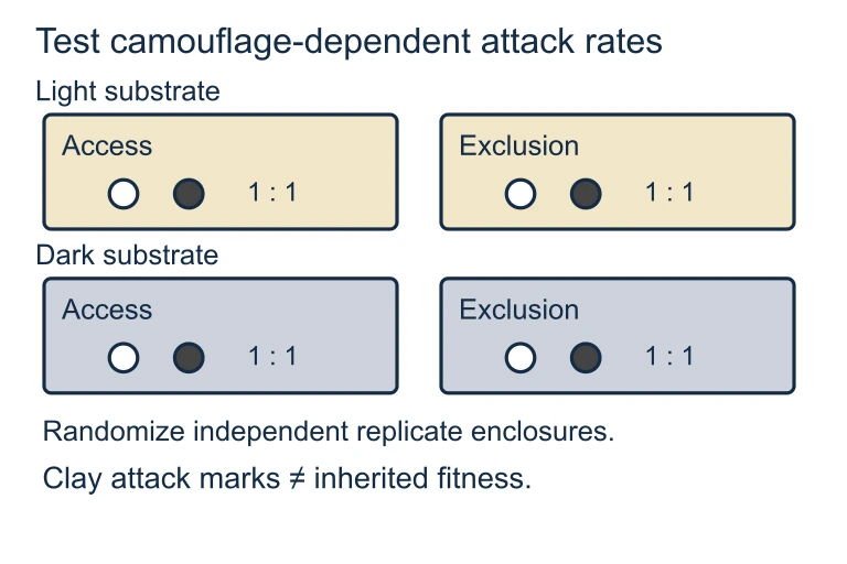Compare light and dark models on both substrates, with predator-access and exclusion treatments. Randomized independent enclosures test camouflage-dependent attack rates; reproductive success requires additional evidence.

SECTION 6

Worked Example: Detecting Selection with Hardy-Weinberg

Consider a population of 500 wildflowers in which flower color is controlled by a single gene with two alleles: C^R (red, dominant) and C^W (white, recessive). A census reveals 320 red-flowered and 180 white-flowered individuals. Determine allele frequencies and assess whether the population is in Hardy-Weinberg equilibrium.

Hardy-Weinberg Analysis of Wildflower Color

1
Step 1 — Identify Given Values

Total population N = 500. Phenotype counts: 320 red (C^RC^R + C^RC^W) and 180 white (C^WC^W). White flowers are homozygous recessive, so white frequency = q².
2
Step 2 — Calculate q from q²

q² = 180 / 500 = 0.36. Taking the square root: q = √0.36 = 0.60.

q = 0.60
3
Step 3 — Calculate p

Since p + q = 1: p = 1 − 0.60 = 0.40.

p = 0.40
4
Step 4 — Predict HWE Genotype Frequencies

Expected frequencies: p² = (0.40)² = 0.16 (homozygous dominant), 2pq = 2 × 0.40 × 0.60 = 0.48 (heterozygotes), q² = 0.36 (homozygous recessive). Expected counts in N = 500: 80 homozygous dominant, 240 heterozygotes, 180 homozygous recessive. Red phenotype expected: 80 + 240 = 320.

Expected: 320 red, 180 white
5
Step 5 — Compare Observed vs. Expected

Observed: 320 red, 180 white. Expected: 320 red, 180 white. The phenotype counts match HWE predictions exactly. However, because dominance masks genotype differences, a chi-square test on genotype data (if available) would be needed to confirm true equilibrium. With only phenotype data, we cannot distinguish whether heterozygote frequency deviates. In this simplified example, the population is consistent with HWE, suggesting no strong selection at this locus—but the inability to distinguish heterozygotes is a limitation of phenotype-only analysis.

Consistent with HWE — no detectable selection using phenotype data alone

ℹ

Why This Matters

If instead we observed 380 red and 120 white flowers, then q² = 0.24, q ≈ 0.49, and p ≈ 0.51, predicting ~380 red and ~120 white—still consistent with HWE for those allele frequencies. A genuine deviation would require genotype data showing, for example, an excess of heterozygotes (suggesting heterozygote advantage) or a deficit (suggesting assortative mating or selection against heterozygotes). This is why molecular tools that distinguish genotypes are essential for detecting selection.

SECTION 7

Selection vs. Other Evolutionary Mechanisms

Natural selection is a powerful evolutionary force, but it is not the only mechanism that changes allele frequencies within populations. The AP Biology exam expects you to distinguish among the five agents of microevolution—natural selection, genetic drift, gene flow, mutation, and nonrandom mating—and to recognize which mechanisms produce adaptive versus non-adaptive change. The table below contrasts natural selection with these other forces along several key dimensions.

Feature	Natural Selection	Genetic Drift	Gene Flow
Directionality	Directional—shifts allele frequencies toward higher fitness	Random—alleles may increase or decrease by chance	Tends to homogenize allele frequencies among populations
Effect on adaptation	The only mechanism that consistently produces adaptation	Can fix deleterious, neutral, or beneficial alleles randomly	May introduce beneficial alleles or disrupt local adaptation
Population-size dependence	Effective in large and small populations	Strongest in small populations (bottlenecks, founder effects)	Depends on migration rate, not population size per se
Genetic variation	Reduces variation at selected loci (directional); maintains it (balancing)	Reduces variation through random fixation or loss	Increases within-population variation; decreases between-population variation
Predictability	Predictable: phenotype-fitness relationships determine outcome	Stochastic: outcomes vary unpredictably among replicates	Semi-predictable: direction depends on source population allele frequencies

Comparison of three major evolutionary mechanisms

✦

KEY TAKEAWAY

Natural selection is sometimes compared to a sculptor working marble: it has a consistent direction dictated by the environment, chipping away less-fit variants to reveal the adaptive form within the raw material of genetic variation. Genetic drift, by contrast, is like an earthquake that randomly chips the marble—it changes the statue's shape, but not toward any particular design. Gene flow is like mixing clay from different sources: it can either enrich the sculptor's material or dilute a regionally refined form. Only selection is inherently adaptive.

SECTION 8

Connecting to Advanced Evolutionary Theory

The modes and mathematics of natural selection covered in this lesson form the bedrock of several advanced topics you may encounter in college-level evolutionary biology or upper-division ecology courses. Understanding how selection at the population level connects to speciation, coevolution, and evo-devo (evolutionary developmental biology) will give you a broader perspective, even though the AP exam focuses primarily on the mechanisms and evidence themselves.

This Lesson	Advanced Extension
Directional selection shifts mean phenotype	Sustained directional selection can drive speciation if isolated populations experience different directional pressures (allopatric divergence)
Disruptive selection produces bimodal distributions	May lead to sympatric speciation if assortative mating evolves between the two phenotypic modes, as modeled in studies of cichlid fishes
Balancing selection (heterozygote advantage)	Maintained polymorphisms can be ancient; trans-species polymorphisms in MHC loci predate the divergence of humans and chimpanzees
Fitness functions determine mode of selection	Adaptive landscapes (Wright's fitness landscapes) formalize how populations navigate peaks and valleys in multidimensional genotype space
Hardy-Weinberg as a null model	Coalescent theory and genome-wide association studies (GWAS) use more sophisticated null models to detect selection at specific genomic loci

Connections between this lesson and advanced evolutionary topics

Looking forward, the integration of genomics with ecology—sometimes called landscape genomics—is allowing researchers to map selection pressures across geographic space and link specific alleles to environmental gradients such as temperature, altitude, or pathogen prevalence. These approaches reinforce that natural selection is not merely a historical concept but an ongoing, measurable process shaping the biodiversity we observe today.

SECTION 9

Practice Problems

Question 1: CONCEPTUAL

A researcher measures beak depth in a finch population before and after a severe drought. After the drought, the mean beak depth has increased, and the distribution has shifted to the right. Which mode of selection is most likely operating?

A. Stabilizing selection
B. Disruptive selection
C. Directional selection
D. Frequency-dependent selection

Show answer (C)

C is correct. A shift of the entire distribution toward one extreme (larger beaks) is the hallmark of directional selection—drought conditions favored birds capable of cracking harder, larger seeds. A (stabilizing selection) would narrow the distribution around the existing mean without shifting it. B (disruptive selection) would produce a bimodal distribution favoring both extremes. D (frequency-dependent selection) describes situations where the fitness of a phenotype depends on its frequency in the population, which is not indicated by a simple mean shift.

Question 2: BASIC CALCULATION

In a population of 1,000 individuals, 40 show the homozygous recessive phenotype (aa). Assuming Hardy-Weinberg equilibrium, what is the expected number of heterozygous (Aa) individuals?

A. 160
B. 320
C. 480
D. 640

Show answer (B)

B is correct. q² = 40/1000 = 0.04, so q = 0.20 and p = 0.80. The heterozygote frequency is 2pq = 2 × 0.80 × 0.20 = 0.32. In 1,000 individuals: 0.32 × 1000 = 320 heterozygotes. A (160) would correspond to 2pq = 0.16, which does not match any correct calculation from these allele frequencies. C (480) and D (640) overestimate the heterozygote count; 480 would require allele frequencies near p = q = 0.5, and 640 exceeds the maximum possible heterozygote frequency of 500 (at p = q = 0.5).

Question 3: INTERMEDIATE

In a population where the sickle-cell allele (HbS) is maintained at a frequency of 0.10 due to heterozygote advantage in malaria-endemic regions, which of the following would most likely occur if malaria were completely eradicated from the region?

A. The frequency of HbS would increase because homozygous HbS individuals would no longer be disadvantaged.
B. The frequency of HbS would decrease because heterozygote advantage would no longer apply, and selection against HbS homozygotes would dominate.
C. The frequency of HbS would remain stable because allele frequencies do not change once equilibrium is reached.
D. Disruptive selection would increase phenotypic variance for hemoglobin type.

Show answer (B)

B is correct. Heterozygote advantage maintains HbS because HbA/HbS individuals have higher fitness than either homozygote in malaria-endemic environments—they resist malaria without suffering sickle-cell disease. If malaria is eradicated, the heterozygote no longer has a fitness advantage over the HbA homozygote, so the balance tips: HbS homozygotes still suffer sickle-cell disease (reduced fitness), and now heterozygotes have no compensating advantage. This shifts to directional selection against HbS, gradually decreasing its frequency. A is incorrect because HbS homozygotes always have reduced fitness due to sickle-cell disease. C is incorrect because equilibrium allele frequencies shift when selective pressures change. D is incorrect because removing malaria does not create a scenario favoring both extremes.

Question 4: APPLIED

4 pts

A population of beetles exhibits variation in exoskeleton color, ranging from light tan to dark brown. You hypothesize that directional selection by bird predators favors darker beetles on dark soil substrates. Design an experiment to test this hypothesis. In your response, include: (a) the independent and dependent variables, (b) the experimental and control groups with appropriate replication, (c) one method to collect data and quantify selection, and (d) a prediction of results if your hypothesis is supported.

Show answer

Point 1 (Variables — 1 pt): The independent variable is substrate color (dark soil vs. light soil). The dependent variable is the survival rate (or frequency change) of beetles in different color categories. A correct response identifies both variables and operationally defines how survival is measured (e.g., proportion surviving after a set time period). Point 2 (Experimental design — 1 pt): Set up replicated field enclosures (minimum 10 per treatment) on dark soil and light soil substrates, each containing equal numbers of light and dark beetles exposed to natural bird predation. Control groups could include enclosures with predator exclusion (mesh covers) on both soil types to measure baseline survival without predation. Randomization and replication are essential. Point 3 (Data collection method — 1 pt): Use mark-recapture methodology, individually marking beetles and censusing survivors at regular intervals (e.g., every 24 hours for 7 days). Calculate relative survival of each color morph on each substrate. Alternatively, measure the change in mean color score (phenotype frequency distribution) over the experimental period. Point 4 (Prediction — 1 pt): If the hypothesis is correct, dark beetles on dark soil should have significantly higher survival rates than light beetles on the same substrate, because crypsis reduces predation. On light soil, the prediction reverses (light beetles survive better), or at minimum, the selective advantage of dark beetles disappears. In predator-exclusion controls, survival should not differ significantly between color morphs, confirming that differential survival is due to predation, not other factors.

Question 5: CRITICAL THINKING

4 pts

A researcher studying a plant population over 10 generations records the frequency of a recessive allele (q) conferring drought tolerance. The data are: Generation 0: q = 0.20 Generation 5: q = 0.35 Generation 10: q = 0.52 The region experienced a persistent multi-year drought beginning just before Generation 0. (a) Describe the trend in allele frequency and identify the most likely mode of selection. (b) Explain why the allele frequency changed as observed, referencing differential fitness. (c) Calculate the expected frequency of homozygous drought-tolerant individuals (qq) at Generation 10 under Hardy-Weinberg assumptions and explain one reason the actual frequency might differ from this expectation. (d) Predict what would happen to q if the drought ended and conditions returned to the historical wet climate.

Show answer

Point 1 (Trend and mode — 1 pt): The frequency of the drought-tolerance allele (q) increased steadily from 0.20 to 0.52 over 10 generations. This is consistent with directional selection favoring the drought-tolerant phenotype. The mean phenotype for drought tolerance is shifting in one direction. Point 2 (Differential fitness explanation — 1 pt): During the drought, individuals homozygous for the drought-tolerance allele (qq) and, to a lesser extent, heterozygous carriers have higher fitness (greater survival and/or reproductive output) than individuals lacking the allele (pp, non-drought-tolerant homozygotes). This differential reproductive success causes the q allele to increase in frequency each generation. The selection coefficient against the non-tolerant phenotype is positive, driving Δq > 0 per generation. Point 3 (HWE calculation and deviation — 1 pt): At Generation 10, q = 0.52, so q² = (0.52)² = 0.2704. Approximately 27% of individuals are expected to be homozygous drought-tolerant. One reason the actual frequency might differ: if the drought creates strong selection, the population is violating the HWE assumption of no selection, and viability selection within each generation could cause observed genotype frequencies to deviate from equilibrium predictions. Additionally, if population size has been reduced by the drought, genetic drift could add stochastic deviation. Point 4 (Prediction if drought ends — 1 pt): If the drought ends and wet conditions return, the selective advantage of the drought-tolerance allele would diminish or disappear. If there is a fitness cost to drought tolerance under wet conditions (e.g., reduced competitive ability, slower growth), directional selection would reverse, gradually decreasing q. If the allele is selectively neutral under wet conditions, q would remain near 0.52 and change only through drift. The rate of any decrease would depend on the magnitude of the selection coefficient against the allele in the new environment.

SUMMARY

Lesson Summary

Summary

This lesson examined how natural selection operates through three primary modes—directional, stabilizing, and disruptive—each reshaping a population's phenotype distribution in a characteristic way dictated by the underlying fitness function. We also explored sexual selection and balancing selection (including heterozygote advantage) as specialized forms that maintain phenotypic diversity or drive the evolution of elaborate traits.

Quantitatively, the Hardy-Weinberg equilibrium serves as a null model: departures from its predictions (p² + 2pq + q² = 1) signal that evolutionary forces such as selection, drift, or gene flow are at work. Five converging lines of evidence—the fossil record, molecular data, biogeography, direct observation, and comparative anatomy—confirm that natural selection is the sole evolutionary mechanism that consistently produces adaptive evolution, distinguishing it from random processes like genetic drift. For the AP exam, focus on identifying modes of selection from phenotype distribution data, applying Hardy-Weinberg calculations, and designing or interpreting experiments that test for selection in natural populations.