Mendelian Genetics - AP Biology

SECTION 1

Historical Context & Motivation

Before the mid-nineteenth century, inheritance was commonly explained by blending inheritance—the idea that offspring traits are simply an intermediate mixture of parental characteristics, much like blending two colors of paint. This model could not explain why traits sometimes skip generations or why offspring occasionally display characteristics absent in both parents. The need for a particulate, predictive framework for heredity set the stage for one of the most transformative experimental programs in the history of biology.

1856 • Mendel Begins Experiments

Gregor Mendel, an Augustinian friar in Brno (modern Czech Republic), begins systematic hybridization experiments with Pisum sativum (garden peas), tracking seven discrete traits across thousands of plants.

1866 • Publication of Results

Mendel publishes "Experiments on Plant Hybridization" in the Proceedings of the Natural History Society of Brünn. The paper introduces the concepts of dominant and recessive factors and proposes precise mathematical ratios for trait inheritance.

1900 • Rediscovery

Hugo de Vries, Carl Correns, and Erich von Tschermak independently rediscover Mendel's work, confirming his ratios in their own plant crosses and launching the modern science of genetics.

1902 • Chromosome Theory

Walter Sutton and Theodor Boveri independently propose that Mendel's "factors" reside on chromosomes, providing the physical basis for segregation and independent assortment during meiosis.

1909 • Term "Gene" Coined

Wilhelm Johannsen introduces the word "gene" to replace Mendel's "factor," along with "genotype" and "phenotype," standardizing the vocabulary of heredity still used today.

Mendel's genius lay in choosing an organism with clearly distinguishable, either-or traits and in applying rigorous quantitative analysis to his results. His central question—how are heritable traits transmitted from one generation to the next?—remains the foundational inquiry of genetics. Understanding his laws is essential before exploring extensions such as polygenic inheritance, epistasis, and the molecular basis of gene expression.

SECTION 2

Core Principles & Definitions

Mendelian genetics rests on several interrelated principles that collectively describe how discrete units of heredity—genes—behave during sexual reproduction. Each gene may exist in alternative forms called alleles. Diploid organisms carry two alleles per gene locus, one inherited from each parent. When both alleles at a locus are identical the organism is homozygous; when they differ the organism is heterozygous. The particular combination of alleles constitutes the genotype, while the observable expression of those alleles is the phenotype.

Law of Dominance

In a heterozygote, one allele (dominant) may mask the expression of another (recessive). The phenotype reflects only the dominant allele.

Law of Segregation

During gamete formation (meiosis), the two alleles for each gene separate equally so that each gamete carries only one allele per locus.

Law of Independent Assortment

Alleles of different genes assort independently during gamete formation, provided the genes reside on different chromosomes or are far apart on the same chromosome.

Test Cross

Crossing an individual of unknown genotype with a homozygous recessive individual reveals the unknown genotype based on the phenotypic ratio of offspring.

SECTION 3

Monohybrid Cross — Visual Explanation

The Punnett square is the standard graphical device for predicting offspring genotype and phenotype ratios from a given cross. The diagram below illustrates a monohybrid cross between two heterozygous parents (Pp × Pp), where P represents the dominant allele for purple flower color and p represents the recessive allele for white flower color in pea plants.

A Punnett square for the cross Pp × Pp produces a 1 : 2 : 1 genotypic ratio (PP : Pp : pp) and a 3 : 1 phenotypic ratio (purple : white). The dominant allele P masks p in heterozygotes.

The Punnett square formalizes the law of segregation by placing each parent's possible gamete types along one axis. Each interior cell represents an equally probable fertilization event. Because each parent can contribute either a P or p allele with equal probability (0.5), the four cells are equiprobable, yielding the expected 1 : 2 : 1 genotypic ratio and, under complete dominance, the classic 3 : 1 phenotypic ratio that Mendel observed in his F₂ generation.

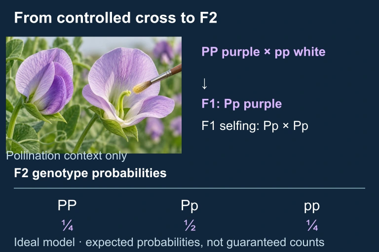Two parents PP and pp converge to F1 Pp. An explicit Pp by Pp self cross gives F2 genotype probabilities one-quarter PP, one-half Pp and one-quarter pp. Maternal anthers are removed before unintended self-pollination, then pollen is transferred from the selected donor. In the simplified model, PP purple × pp white produces purple F1 Pp; intentional F1 selfing gives expected F2 probabilities ¼ PP, ½ Pp, ¼ pp, not guaranteed family counts.

SECTION 4

Mathematical Framework

Mendelian inheritance is inherently probabilistic. The rules of probability—specifically the multiplication rule (for independent events occurring together) and the addition rule (for mutually exclusive events)—allow us to calculate expected genotype and phenotype frequencies without drawing every Punnett square.

MULTIPLICATION RULE (AND)

P(A and B) = P(A) × P(B)

Used when two independent events must both occur. For example, the probability that an offspring receives allele P from parent 1 and allele p from parent 2 is 0.5 × 0.5 = 0.25.

ADDITION RULE (OR)

P(A or B) = P(A) + P(B)

Used when either of two mutually exclusive outcomes satisfies the condition. For instance, the probability of a heterozygote (Pp) from Pp × Pp is P(P from parent 1 and p from parent 2) + P(p from parent 1 and P from parent 2) = 0.25 + 0.25 = 0.50.

DIHYBRID EXPECTED RATIO

9 : 3 : 3 : 1

The phenotypic ratio from a dihybrid cross (AaBb × AaBb) under complete dominance and independent assortment. 9/16 show both dominant phenotypes, 3/16 show dominant for trait A and recessive for trait B, 3/16 the reverse, and 1/16 show both recessive phenotypes.

CHI-SQUARE GOODNESS-OF-FIT

χ² = Σ [(observed − expected)² / expected]

Determines whether deviations between observed and expected offspring counts are due to chance or indicate a statistically significant departure from the Mendelian model. Compare the calculated χ² value to the critical value at p = 0.05 with the appropriate degrees of freedom (df = number of phenotypic classes − 1).

ℹ

AP Exam Tip

SECTION 5

Dihybrid Cross & Independent Assortment

Mendel extended his analysis from single-trait (monohybrid) crosses to two-trait (dihybrid) crosses. When he crossed plants heterozygous for both seed shape (Rr) and seed color (Yy), the F₂ generation displayed a 9 : 3 : 3 : 1 phenotypic ratio. This result confirmed that alleles of different genes assort independently during meiosis—the Law of Independent Assortment.

A 4 × 4 Punnett square for the dihybrid cross RrYy × RrYy. The 9 : 3 : 3 : 1 phenotypic ratio results from the independent assortment of two gene loci on separate chromosomes.

The 9 : 3 : 3 : 1 ratio is a direct consequence of multiplying two independent 3 : 1 ratios: (3 : 1) × (3 : 1) = 9 : 3 : 3 : 1. Any significant deviation from this ratio in experimental data—testable via the chi-square statistic—may indicate that the two genes are linked on the same chromosome or that another non-Mendelian mechanism is operating.

SECTION 6

Worked Example — Chi-Square Analysis

A researcher crosses two heterozygous pea plants (Pp × Pp) and observes the following among 200 offspring: 160 purple-flowered and 40 white-flowered. Do these data support the expected 3 : 1 Mendelian ratio at a significance level of 0.05?

Worked example

1
Step 1 — State the Null Hypothesis

H₀: The observed offspring ratio does not differ significantly from the expected 3 : 1 ratio. Any deviation is due to chance alone.
2
Step 2 — Calculate Expected Values

With 200 total offspring and a 3 : 1 ratio, the expected counts are: Purple = (3/4) × 200 = 150; White = (1/4) × 200 = 50.

Expected: 150 purple, 50 white
3
Step 3 — Compute χ² for Each Class

Purple: (160 − 150)² / 150 = 100 / 150 = 0.667. White: (40 − 50)² / 50 = 100 / 50 = 2.000.
4
Step 4 — Sum to Get Total χ²

χ² = 0.667 + 2.000 = 2.667. Degrees of freedom = number of phenotypic classes − 1 = 2 − 1 = 1.

χ² = 2.667, df = 1
5
Step 5 — Compare to Critical Value

The critical value for χ² with 1 df at p = 0.05 is 3.841. Because 2.667 < 3.841, we fail to reject H₀. The observed data are consistent with a 3 : 1 Mendelian ratio; deviations can be attributed to random sampling variation.

Conclusion: Data support the Mendelian 3 : 1 ratio.

SECTION 7

Strengths & Limitations of Mendelian Genetics

Strengths	Limitations
Provides a simple, predictive mathematical framework for discrete traits governed by single genes.	Cannot explain continuous (quantitative) traits controlled by many genes (polygenic inheritance).
Accurately describes complete dominance, which occurs for many loci across diverse organisms.	Does not account for incomplete dominance, codominance, or multiple alleles at a single locus.
Independent assortment correctly predicts outcomes for genes on separate chromosomes.	Fails for linked genes on the same chromosome, where recombination frequency varies with map distance.
Test crosses allow determination of unknown genotypes, a powerful tool in breeding and research.	Ignores environmental influences on phenotype, epistasis, pleiotropy, and epigenetic modifications.

Mendelian genetics excels for single-gene traits with complete dominance but must be extended for many real-world inheritance patterns.

SECTION 8

Connection to Non-Mendelian & Molecular Genetics

Feature	Mendelian (Classical)	Non-Mendelian / Molecular
Allele interactions	Complete dominance; two alleles per locus	Incomplete dominance, codominance, multiple alleles (e.g., ABO blood types with Iᴬ, Iᴮ, i)
Number of genes per trait	One gene → one phenotype	Polygenic traits (e.g., skin color, height); pleiotropy (one gene → many phenotypes)
Gene interaction	Genes act independently	Epistasis: one gene masks or modifies expression of another gene (e.g., Labrador coat color)
Chromosome behavior	Independent assortment assumed	Linked genes on the same chromosome; recombination frequency used for gene mapping
Inheritance pattern	Autosomal; sex not considered	Sex-linked inheritance (X-linked traits), mitochondrial inheritance, genomic imprinting

Mendelian vs. Non-Mendelian genetics comparison

As you progress through the AP Biology curriculum, you will encounter these extensions in depth. The chromosome theory of inheritance, confirmed by Thomas Hunt Morgan's work with Drosophila, showed that genes are physically located on chromosomes, explaining why some genes violate independent assortment. Later, Watson and Crick's elucidation of DNA structure provided the molecular basis for how alleles encode different polypeptides. Each of these advances is an extension of—not a departure from—Mendel's original insight that heredity is governed by discrete, particulate factors.

SECTION 9

Practice Problems

Question 1: CONCEPTUAL

In pea plants, tall (T) is dominant over short (t). A heterozygous tall plant is crossed with a short plant. What is the expected phenotypic ratio of the offspring?

A. All tall
B. 3 tall : 1 short
C. 1 tall : 1 short
D. 1 tall : 3 short

Show answer (C)

C is correct. The cross Tt × tt produces gametes T and t from the heterozygous parent and only t from the homozygous recessive parent. The resulting offspring are 1/2 Tt (tall) and 1/2 tt (short), yielding a 1 : 1 phenotypic ratio. A is wrong because "all tall" would result from TT × tt, where every offspring is Tt. B is wrong because a 3 : 1 ratio results from Tt × Tt (two heterozygotes), not a test cross. D is wrong because it inverts the ratio; a dominant allele from one parent ensures at least half the offspring are tall.

Question 2: BASIC CALCULATION

In a cross between two organisms heterozygous for two independently assorting genes (AaBb × AaBb), what is the probability of an offspring with the genotype AABb?

A. 1/16
B. 1/8
C. 3/16
D. 1/4

Show answer (B)

B is correct. Using the multiplication rule for independent events: P(AA) = 1/4 (from Aa × Aa) and P(Bb) = 2/4 = 1/2 (from Bb × Bb). Therefore P(AABb) = 1/4 × 1/2 = 1/8. A (1/16) is the probability of AABB, not AABb. C (3/16) does not correspond to any single genotype probability in this cross. D (1/4) is the probability of AA alone, ignoring the B locus entirely.

Question 3: INTERMEDIATE

A researcher crosses a purple-flowered pea plant with a white-flowered pea plant and obtains 52 purple and 48 white offspring. Which of the following is the most likely genotype of the purple parent?

A. PP
B. Pp
C. pp
D. Either PP or Pp; the data cannot distinguish them

Show answer (B)

B is correct. The white parent must be pp (homozygous recessive). The offspring ratio of approximately 1 : 1 purple to white indicates a test cross. If the purple parent were PP (choice A), all offspring would be Pp and therefore purple; no white offspring would appear. Choice C is impossible because a pp plant has white flowers, not purple. Choice D is wrong because the data clearly distinguish the two: a PP parent produces 100% purple offspring, whereas a Pp parent produces the observed ~1 : 1 ratio. This is the classic test cross pattern.

Question 4: APPLIED

A biologist has a population of fruit flies (Drosophila melanogaster) exhibiting wild-type body color. The biologist hypothesizes that some flies may be heterozygous carriers of the recessive ebony body allele (e). Design an experiment to test this hypothesis. In your response: (a) Describe the cross you would perform and explain why it is appropriate. (b) State the expected phenotypic ratios if the hypothesis is correct. (c) State the expected phenotypic ratios if the hypothesis is incorrect (i.e., the wild-type flies are homozygous). (d) For the heterozygous-parent hypothesis, explain how to test a 1:1 expected ratio using chi-square when expected counts are adequate. Include the null hypothesis, degrees of freedom and decision criterion. Explain why this calculation is not valid for a 1:0 expected ratio and how to interpret the absence of ebony offspring in a finite sample.

Show answer

(a) Perform a test cross by mating each suspected wild-type fly with a homozygous ebony fly (ee). The test cross is appropriate because the homozygous recessive parent can only contribute the recessive allele, so the offspring phenotype directly reveals the allele contributed by the wild-type parent. (b) If the wild-type parent is heterozygous (Ee), the cross Ee × ee produces 1/2 Ee (wild-type) : 1/2 ee (ebony), a 1 : 1 phenotypic ratio. (c) If the wild-type parent is homozygous (EE), the cross EE × ee produces 100% Ee offspring, all wild-type. No ebony offspring would appear. (d) Under the heterozygous-parent null hypothesis, the expected ratio is 1:1, so E = N/2 in each of the two classes. With adequate expected counts, calculate χ² = Σ[(O − E)²/E], with df = 1. At α = 0.05, reject this null if χ² > 3.841. For a 1:0 ratio, one expected count is zero, so this chi-square statistic is undefined. Under the ideal complete-dominance/no-error model, an ebony offspring contradicts EE parentage. If no ebony offspring appear, the probability of that outcome under Ee is

(1/2)^N

; absence in a finite sample does not prove homozygosity. Scoring errors or incomplete penetrance, if assumed, require separate consideration.

Question 5: CRITICAL THINKING

A student performs a dihybrid cross (BbRr × BbRr) in plants where B = brown seed (dominant) and R = round seed (dominant). The student observes the following F₂ data from 640 offspring: • Brown, Round: 360 • Brown, Wrinkled: 130 • Green, Round: 120 • Green, Wrinkled: 30 (a) Calculate the expected number of offspring in each phenotypic class assuming a 9:3:3:1 ratio. (b) Perform a chi-square analysis on these data. (c) With 3 degrees of freedom and a critical value of 7.815 at p = 0.05, state whether the null hypothesis should be rejected. (d) Propose a biological explanation for any deviation from the expected ratio.

Show answer

(a) Expected values based on 9:3:3:1 ratio with n = 640: Brown Round = 9/16 × 640 = 360; Brown Wrinkled = 3/16 × 640 = 120; Green Round = 3/16 × 640 = 120; Green Wrinkled = 1/16 × 640 = 40. (b) χ² = (360 − 360)²/360 + (130 − 120)²/120 + (120 − 120)²/120 + (30 − 40)²/40 = 0 + 0.833 + 0 + 2.5 = 3.333. (c) With df = 4 − 1 = 3 and a critical value of 7.815 at p = 0.05, χ² = 3.333 < 7.815. We fail to reject the null hypothesis. The data are statistically consistent with the expected 9:3:3:1 Mendelian dihybrid ratio. (d) Although the null is not rejected, the observed deficit of green wrinkled seeds (30 vs. 40 expected) and slight excess of brown wrinkled (130 vs. 120) could be due to random sampling variation. Alternatively, partial gene linkage could slightly alter expected ratios, or differential seed viability could cause some genotypes to be underrepresented. Repeating the experiment with a larger sample size would help distinguish random variation from a biologically meaningful departure.