Effect of Density on Populations - AP Biology

SECTION 1

Historical Context & Motivation

The question of what limits the growth of natural populations has occupied ecologists for centuries. Early naturalists observed that no species expands infinitely, yet the mechanisms constraining population size remained elusive. The intellectual trajectory from Thomas Malthus's demographic warnings in the late 18th century to modern mathematical ecology traces a progressive understanding that population density itself acts as a feedback signal regulating growth. Understanding density-dependent and density-independent factors is essential to predicting how populations change over time—a core objective of AP Biology's ecology unit.

1798 • Malthus's Essay on Population

Thomas Malthus argues that human populations grow geometrically while resources grow arithmetically, predicting inevitable checks such as famine and disease.

1838 • Verhulst's Logistic Equation

Pierre-François Verhulst introduces the logistic growth model, incorporating carrying capacity (K) as the environmental ceiling on population size.

1920s • Lotka-Volterra Models

Alfred Lotka and Vito Volterra independently develop mathematical models of predator-prey and competition dynamics, formalizing density-dependent interactions between species.

1954 • Lack's Regulation of Animal Numbers

David Lack demonstrates that food supply and territorial behavior limit bird populations in a density-dependent manner, grounding theory in empirical observation.

1970s–Present • Modern Population Ecology

Ecologists integrate density-dependent and density-independent factors with stochastic models, metapopulation theory, and climate change projections to manage wildlife and conservation.

The central question motivating this lesson is straightforward yet profound: why don't populations grow forever, and what role does population density play in regulating their size? Answering this question requires distinguishing between factors that intensify as density rises and those that strike regardless of how many individuals are present.

SECTION 2

Core Principles & Definitions

Population ecology distinguishes two broad categories of factors that influence population growth rate: those whose effects scale with the number of individuals per unit area (density-dependent factors) and those whose impact is unrelated to crowding (density-independent factors). Together, these two classes of regulation determine whether a population stabilizes near its carrying capacity (K), crashes, or fluctuates unpredictably.

Density-Dependent Regulation

Factors whose per-capita effect intensifies as population density increases. Examples include intraspecific competition for food, predation, disease transmission, and waste accumulation.

Density-Independent Factors

Environmental events that reduce populations regardless of size—natural disasters (floods, fires, hurricanes), seasonal temperature extremes, and human habitat destruction.

Carrying Capacity (K)

The maximum population size that an environment can sustain indefinitely given available resources, space, and other ecological constraints. K is not fixed—it shifts with environmental conditions.

Logistic Growth

A model describing population growth that slows as N approaches K, producing an S-shaped (sigmoidal) curve. The term (K − N)/K represents density-dependent feedback.

Negative Feedback Loop

As density rises, per-capita birth rates decline and/or death rates increase, pushing the population back toward K. This self-correcting mechanism is the hallmark of density-dependent regulation.

SECTION 3

Visual Explanation — Growth Curves Compared

The pink J-shaped curve represents exponential growth (dN/dt = rN), which occurs when resources are unlimited. The cyan S-shaped curve represents logistic growth (dN/dt = rN(K − N)/K), where the growth rate slows as N approaches the carrying capacity K (amber dashed line). At low densities both curves are nearly identical; they diverge as density-dependent feedback intensifies.

The diagram above illustrates the fundamental distinction between growth with and without density regulation. In the exponential model, per-capita growth rate remains constant regardless of N, leading to a J-curve that accelerates without bound. In the logistic model, the term (K − N)/K approaches zero as N nears K, causing the population growth rate to decline. When N = K, the population is at equilibrium and net growth is zero. When N exceeds K, the term becomes negative, meaning deaths exceed births and the population shrinks—a clear demonstration of negative feedback.

SECTION 4

Mathematical Framework

Two equations form the mathematical backbone of population growth modeling on the AP Biology exam. Mastering the relationship between them reveals how density-dependent regulation is encoded algebraically.

EXPONENTIAL GROWTH

dN/dt = r_max × N

N = population size; r_max = maximum per-capita growth rate (intrinsic rate of increase); dN/dt = change in N over time. No carrying capacity term exists, so growth accelerates without limit.

LOGISTIC GROWTH

dN/dt = r_max × N × (K − N) / K

K = carrying capacity. The factor (K − N)/K is the density-dependent modifier. When N is small relative to K, (K − N)/K ≈ 1 and growth resembles exponential. When N = K, (K − N)/K = 0 and growth halts. When N > K, the modifier is negative and the population declines.

MAXIMUM GROWTH RATE

Maximum dN/dt occurs when N = K / 2

The logistic curve's inflection point—where the population grows fastest—occurs at half the carrying capacity. This result is derived by differentiating the logistic equation with respect to N and setting the second derivative to zero. This is a frequently tested concept on the AP exam.

The elegance of the logistic model lies in its simplicity: a single multiplicative term converts unchecked exponential growth into regulated, density-dependent growth. However, real populations often overshoot K, oscillate, or experience time-lagged density effects, which is why more complex models exist. For the AP exam, it is critical to understand that the logistic model captures the idealized effect of density on population growth rate.

SECTION 5

Density-Dependent vs. Density-Independent Factors

Understanding the contrast between density-dependent and density-independent factors is essential for interpreting population data on the AP exam. Density-dependent factors create a negative feedback loop that stabilizes populations, while density-independent factors produce mortality or reduced reproduction that does not vary with N.

Density-dependent factors (left, violet) intensify with crowding and produce stabilizing negative feedback. Density-independent factors (right, orange) impact populations regardless of size and do not create regulatory feedback loops.

A key nuance tested on the AP exam is that density-dependent factors regulate populations (push them toward K), whereas density-independent factors merely limit or reduce them without creating a self-correcting trajectory. Both categories can act simultaneously on the same population: a drought (density-independent) may reduce food supply, lowering K, which intensifies competition (density-dependent). This interplay makes real ecological systems complex but also makes exam questions that require you to classify factors particularly common.

ℹ

AP Exam Tip

SECTION 6

Worked Example — Logistic Growth Calculation

Consider a population of white-tailed deer in a managed forest. The carrying capacity is estimated at K = 500 individuals. The current population size is N = 130, and the intrinsic rate of increase is r_max = 0.5 per year. Calculate the population growth rate (dN/dt) and determine whether the population is growing at its maximum possible rate.

Worked example

1
Step 1 — Identify Given Values

N = 130 deer, K = 500 deer, r_max = 0.5 per year.
2
Step 2 — Write the Logistic Equation

dN/dt = r_max × N × (K − N) / K
3
Step 3 — Substitute Values

dN/dt = 0.5 × 130 × (500 − 130) / 500 = 0.5 × 130 × 370 / 500
4
Step 4 — Calculate Step by Step

(K − N)/K = 370/500 = 0.74. Then dN/dt = 0.5 × 130 × 0.74 = 65 × 0.74 = 48.1 deer per year.

dN/dt = 48.1 deer/year
5
Step 5 — Evaluate Maximum Growth

Maximum dN/dt occurs at N = K/2 = 250. At N = 250: dN/dt = 0.5 × 250 × (500 − 250)/500 = 0.5 × 250 × 0.5 = 62.5 deer/year. Because N = 130 < 250, the population is not yet at its maximum growth rate. The current rate of 48.1 deer/year is below the theoretical maximum of 62.5 deer/year.

Maximum dN/dt = 62.5 deer/year at N = 250

SECTION 7

Strengths & Limitations of the Logistic Model

Aspect	Strength	Limitation
Simplicity	Uses only N, K, and r — easy to parameterize and teach	Oversimplifies; real populations face multiple interacting factors
Density Feedback	Captures the essential negative feedback as N → K	Assumes instantaneous response; ignores time lags that cause oscillations
Carrying Capacity	Introduces the concept of environmental limits on growth	Treats K as fixed; in reality K fluctuates with seasons, climate, and resources
Predictions	Predicts S-shaped growth—matches many real organisms (yeast, bacteria, Paramecium)	Fails for populations that overshoot K, exhibit boom-bust cycles, or have Allee effects
Species Interactions	Foundation for Lotka-Volterra competition and predator-prey models	Ignores interspecific competition, mutualism, and community-level dynamics

Strengths and limitations of the logistic growth model

SECTION 8

Connection to Advanced Ecological Theory

The logistic model serves as the conceptual gateway to more sophisticated population and community ecology frameworks. Understanding how density effects shape growth prepares you for topics ranging from life-history strategy theory to conservation biology.

Concept from This Lesson	Advanced Extension
Density-dependent competition	r/K selection theory — species adapted to uncrowded vs. crowded environments invest differently in reproduction and survivorship
Logistic growth with fixed K	Lotka-Volterra competition — two species share resources; the competition coefficient α modifies each species' K based on the other's density
Predation as density-dependent mortality	Lotka-Volterra predator-prey — coupled differential equations model oscillating prey and predator densities
Negative feedback near K	Allee effect — at very low densities, per-capita growth can decrease (positive density dependence), threatening small populations with extinction
Population regulation	Metapopulation dynamics — multiple subpopulations connected by migration; local extinctions and recolonizations are density-influenced

How density-dependent concepts extend into advanced ecology

The AP exam will not require you to derive Lotka-Volterra equations, but understanding that density-dependent regulation underlies interspecific competition, predator-prey cycling, and even conservation management (e.g., maximum sustainable yield at N = K/2) gives you the conceptual depth to tackle any related free-response prompt. The take-home message is that the simple logistic equation is the seed from which an entire field of quantitative ecology grows.

SECTION 9

Practice Problems

Question 1: CONCEPTUAL

A population of rabbits in a meadow experiences increased disease transmission as the population grows larger. This is best classified as which type of factor?

A. Density-independent, because disease can occur at any population size
B. Density-dependent, because the rate of transmission increases with crowding
C. Density-independent, because the pathogen is an abiotic factor
D. Density-dependent, because disease always eliminates the same percentage of individuals

Show answer (B)

B is correct because disease transmission rate increases with population density—individuals are in closer contact, allowing pathogens to spread more rapidly, which is the defining characteristic of a density-dependent factor. A is wrong because while disease can occur at any size, the question specifies that transmission increases with population size, making it density-dependent. C is wrong because pathogens are biotic, not abiotic, factors. D is wrong because density-dependent disease does not kill a fixed percentage regardless of density; the per-capita mortality rate from disease increases as density rises.

Question 2: BASIC CALCULATION

A bacterial population has r_max = 1.0 per hour, K = 10,000, and current N = 2,500. What is the population growth rate (dN/dt)?

A. 1,875 bacteria/hour
B. 2,500 bacteria/hour
C. 7,500 bacteria/hour
D. 625 bacteria/hour

Show answer (A)

A is correct. dN/dt = r_max × N × (K − N)/K = 1.0 × 2,500 × (10,000 − 2,500)/10,000 = 2,500 × 0.75 = 1,875. B (2,500) is the result of using the exponential equation (r × N) without the density-dependent modifier. C (7,500) results from incorrectly computing (K − N) without dividing by K. D (625) could result from miscalculating the modifier as 0.25 instead of 0.75.

Question 3: INTERMEDIATE

A population of fish in a lake has K = 800 and r_max = 0.4 per year. At which population size will the growth rate (dN/dt) be greatest, and what will that maximum growth rate be?

A. N = 400; dN/dt = 80 fish/year
B. N = 800; dN/dt = 0 fish/year
C. N = 200; dN/dt = 60 fish/year
D. N = 400; dN/dt = 160 fish/year

Show answer (A)

A is correct. Maximum dN/dt occurs at N = K/2 = 400. At N = 400: dN/dt = 0.4 × 400 × (800 − 400)/800 = 0.4 × 400 × 0.5 = 80 fish/year. B is wrong because at N = K the growth rate is zero, not maximum. C is wrong because while dN/dt at N = 200 is indeed 0.4 × 200 × 0.75 = 60, this is not the maximum—the maximum occurs at K/2. D is wrong because it omits the density-dependent modifier; 160 = 0.4 × 400, which is the exponential growth rate without the (K − N)/K term.

Question 4: APPLIED

A team of ecologists hypothesizes that intraspecific competition for nesting sites is the primary density-dependent factor limiting a population of cavity-nesting birds in a forest. Design an experiment to test this hypothesis. In your response: (a) State a testable prediction. (b) Describe the experimental and control groups, including how you would manipulate the independent variable. (c) Identify two variables that must be controlled and explain why. (d) Describe what data you would collect and how the results would support or refute the hypothesis.

Show answer

(a) Prediction: If nesting site competition is the primary density-dependent factor, then experimentally increasing nest site availability will increase per-capita reproductive success and population growth rate. (1 pt) (b) Experimental design: Select two comparable forest plots with similar initial densities of the target bird species. In the experimental plot, install a large number of artificial nest boxes sufficient to eliminate competition for cavities. The control plot receives no nest boxes. Replicate across multiple paired plots for statistical power. (1 pt) (c) Controlled variables: (i) Food availability—select plots with similar vegetation structure and invertebrate abundance, because food limitation is another density-dependent factor that could confound results. (ii) Predator pressure—ensure both plots have similar predator communities, because differential predation could independently affect reproductive success. (1 pt) (d) Data collection: Record the number of occupied nests, clutch size, hatching success, fledging rate, and population counts at the start and end of each breeding season for at least 3 years. Compare per-capita reproductive output and population growth rate between experimental and control plots using appropriate statistical tests (e.g., t-test or ANOVA). (1 pt) Interpretation: If the experimental group shows statistically significantly higher reproduction and population growth, the hypothesis that nesting site competition is the primary density-dependent limiter is supported. If no significant difference is found, other factors (e.g., food, disease) may play a more dominant role. (1 pt)

Question 5: CRITICAL THINKING

Researchers tracked a population of Paramecium in a laboratory culture over 20 days. The data are below: Day 0: N = 10 Day 2: N = 30 Day 4: N = 80 Day 6: N = 170 Day 8: N = 300 Day 10: N = 420 Day 12: N = 480 Day 14: N = 500 Day 16: N = 510 Day 18: N = 500 Day 20: N = 500 (a) Identify the type of growth curve these data represent and justify your answer. (b) Estimate the carrying capacity (K) of this culture system and explain how you determined it. (c) Between which two-day interval was the population growth rate (ΔN/Δt) greatest? Show your calculation. (d) Explain, using the logistic equation, why the growth rate was highest during that interval rather than earlier or later.

Show answer

(a) The data represent logistic (sigmoidal) growth. The population initially grows rapidly (Days 0–8) but then the rate of increase slows dramatically as N approaches approximately 500, where it stabilizes. This S-shaped pattern is characteristic of density-dependent regulation, unlike exponential growth which would continue accelerating. (1 pt) (b) K ≈ 500 Paramecium. From Day 14 onward, the population stabilizes at approximately 500 with no further net growth, indicating that births equal deaths at this density—the definition of carrying capacity. (1 pt) (c) Calculating ΔN/Δt for each interval: Days 0–2: (30−10)/2 = 10/day; Days 2–4: (80−30)/2 = 25/day; Days 4–6: (170−80)/2 = 45/day; Days 6–8: (300−170)/2 = 65/day; Days 8–10: (420−300)/2 = 60/day; Days 10–12: (480−420)/2 = 30/day; Days 12–14: (500−480)/2 = 10/day. The greatest growth rate is during Days 6–8, with ΔN/Δt = 65 Paramecium per day. (1 pt) (d) According to the logistic equation dN/dt = r_max × N × (K − N)/K, the growth rate is maximized when N = K/2 = 250. During Days 6–8, the population passes through N = 170 to N = 300, which brackets the value K/2 = 250. Earlier in the experiment (e.g., Days 0–4), N was small, so although (K−N)/K was close to 1, the product r × N was small, limiting overall growth rate. Later (e.g., Days 10–14), N was close to K, so (K−N)/K approached zero, again reducing the growth rate. The interval around N = K/2 maximizes the product of both terms. (1 pt)

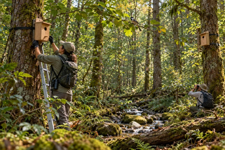
Forest field scene shows installed boxes and monitoring. Visible birds and boxes are contextual rather than measured plot counts or outcomes. Independent forest plots are the treatment replicates in a nest-box experiment. Record reproductive output as well as occupancy, because immigration can increase occupancy without increasing reproduction.

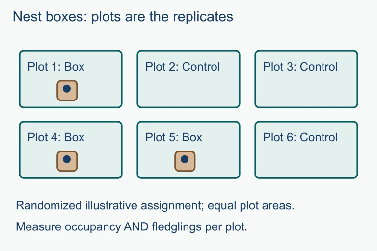
Nest boxes: plots are the replicates. Independent forest plots are the treatment replicates in a nest-box experiment. Record reproductive output as well as occupancy, because immigration can increase occupancy without increasing reproduction. Independent forest plots are the treatment replicates in a nest-box experiment. Record reproductive output as well as occupancy, because immigration can increase occupancy without increasing reproduction.