Disruptions in Ecosystems - AP Biology

SECTION 1

Historical Context & Motivation

Ecologists have long recognized that ecosystems are not static, self-perpetuating entities but dynamic systems shaped by periodic disturbances. Early naturalists such as Charles Darwin observed that volcanic eruptions, storms, and human land use profoundly altered species assemblages, yet it was not until the twentieth century that ecology developed formal frameworks for understanding how disruptions restructure biological communities. The question that drove this field was deceptively simple: why do some ecosystems recover from catastrophic disturbance while others shift to entirely new states?

1916 • Clements's Succession Model

Frederic Clements proposed the concept of ecological succession, arguing that disturbed communities progress through predictable seral stages toward a stable climax community. His organismic metaphor dominated ecology for decades.

1958 • Whittaker's Individualistic Continuum

Robert Whittaker's gradient analysis showed that species respond individually to environmental conditions rather than as tightly co-evolved units, challenging the deterministic view of post-disturbance recovery.

1978 • Connell's Intermediate Disturbance Hypothesis

Joseph Connell argued that species diversity peaks at intermediate levels of disturbance—too little disturbance allows competitive exclusion, while too much eliminates slow colonizers. This hypothesis reframed disruptions as potential drivers of biodiversity.

1980 • Mount St. Helens Eruption

The catastrophic eruption of Mount St. Helens provided ecologists with a large-scale natural experiment in primary succession, yielding decades of data on biological recovery after volcanic devastation.

2005 • Millennium Ecosystem Assessment

This UN-backed report quantified how anthropogenic disruptions—habitat destruction, pollution, climate change, overexploitation, and invasive species—are degrading ecosystem services worldwide at unprecedented rates.

These milestones reveal a fundamental shift in ecological thinking: disturbances are not merely destructive events from which ecosystems must "heal," but integral forces that shape species composition, nutrient cycling, and energy flow. The central question for AP Biology is how disruptions—ranging from fires and floods to invasive species and climate change—alter the structure and function of ecological communities, and what determines whether an ecosystem can recover or transitions to a novel state.

SECTION 2

Core Principles & Definitions

An ecosystem disruption is any event or process that significantly alters the structure, composition, or function of a biological community and its abiotic environment. Disruptions vary in origin (natural versus anthropogenic), scale (local versus global), intensity, frequency, and duration. Understanding these dimensions is essential because the same type of disturbance can have drastically different outcomes depending on its specific characteristics and the resilience of the affected community.

Resistance

The ability of an ecosystem to withstand a disturbance without significant change in species composition, trophic structure, or nutrient cycling. High biodiversity often confers greater resistance through functional redundancy among species.

Resilience

The rate and completeness with which an ecosystem returns to its pre-disturbance state. Resilient systems recover quickly because surviving organisms or seed banks allow rapid recolonization and restoration of trophic interactions.

Ecological Succession

The orderly progression of community change following a disturbance. Primary succession occurs on newly exposed substrates (bare rock, lava), while secondary succession occurs where soil and biological legacies remain.

Keystone & Foundation Species

Keystone species exert disproportionate control over community structure relative to their abundance (e.g., sea otters). Foundation species (e.g., corals) physically create habitat. Loss of either dramatically disrupts the ecosystem.

Trophic Cascades

Indirect effects that propagate through food webs when a disruption removes or adds a species at one trophic level, causing reciprocal changes in abundance at other levels. Top-down cascades (predator removal) are the most well-documented.

SECTION 3

Trophic Cascade — Visual Explanation

One of the most instructive examples of ecosystem disruption is the trophic cascade triggered by the removal or reintroduction of an apex predator. The diagram below illustrates how the loss of wolves from Yellowstone National Park allowed elk populations to explode, leading to overgrazing of riparian vegetation, bank erosion, and declines in songbird and beaver populations. When wolves were reintroduced in 1995, the cascade reversed: elk browsing pressure decreased, willows and aspens regenerated along streams, beavers returned, and the physical structure of the river channels changed—demonstrating that a single disruption at the top of a food web can reshape an entire landscape.

The left column traces the top-down cascade following wolf removal: elk overgrazing degrades riparian vegetation, which in turn eliminates beaver and songbird habitat and destabilizes stream banks. The right column shows the reversal after wolf reintroduction—a classic example of how a single disruption at one trophic level propagates across the entire ecosystem.

This Yellowstone case study illustrates a critical AP Biology concept: disruptions do not remain confined to the trophic level where they originate. The removal of a single apex predator triggered changes that cascaded through herbivores, primary producers, other consumer species, and even the physical landscape. This interconnectedness is precisely why ecologists emphasize the importance of food-web complexity and biodiversity: the more pathways exist for energy and nutrients to flow, the more buffered the system is against the loss of any single component.

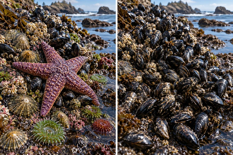Foreground sea star has five arms; left rock contains several sessile forms while right is mussel dominated. Composition is a conceptual comparison, not historical data. Separate exact panel: Two negative causal links connect sea stars to mussels and mussels to other sessile taxa, yielding a positive indirect effect on other taxa. Sea-star predation can reduce mussel dominance and indirectly release other sessile species from competition. A removal experiment compares treated and control plots through time.

A predator can release competitors. Sea-star predation can reduce mussel dominance and indirectly release other sessile species from competition. A removal experiment compares treated and control plots through time. 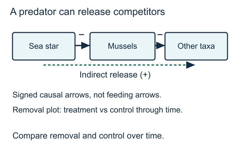Sea-star predation can reduce mussel dominance and indirectly release other sessile species from competition. A removal experiment compares treated and control plots through time.

SECTION 4

Mechanisms of Ecosystem Disruption

Ecosystem disruptions operate through several interrelated mechanisms that alter the flow of energy, the cycling of matter, and the interactions among species. While the AP Biology curriculum does not emphasize extensive mathematical modeling of disruptions, understanding a few quantitative relationships helps clarify why some disturbances have outsized effects.

Energy Flow & Net Primary Productivity

NET PRIMARY PRODUCTIVITY

NPP = GPP − R_a

NPP = net primary productivity (energy available to consumers); GPP = gross primary productivity (total photosynthetic output); R_a = autotrophic respiration. Disruptions that reduce producer biomass (deforestation, herbicide runoff) directly decrease NPP, limiting energy available to all higher trophic levels.

TROPHIC EFFICIENCY

Trophic Efficiency = (Production at level n) / (Production at level n−1) × 100%

Typically ~10% between successive trophic levels. Because energy transfer is so inefficient, disruptions at lower trophic levels (e.g., loss of primary producers) have magnified effects on higher-level consumers that depend on a progressively smaller fraction of the original energy input.

Bioaccumulation & Biomagnification

BIOMAGNIFICATION FACTOR

BMF = [Toxin] in consumer / [Toxin] in prey

A BMF > 1 indicates biomagnification: the toxin is accumulating at higher concentrations in each successive trophic level. DDT famously reached BMFs exceeding 10⁶ in apex predators like peregrine falcons, causing eggshell thinning and population collapse.

Invasive Species & Competitive Displacement

When an invasive species enters an ecosystem, it often lacks natural predators, parasites, or pathogens that regulate its population in its native range—a phenomenon termed enemy release. The competitive exclusion principle predicts that two species competing for identical resources cannot coexist indefinitely; the invader may outcompete native species for food, nesting sites, or light. In addition, invasive species may alter nutrient cycles (e.g., nitrogen-fixing plants enriching previously nutrient-poor soils), facilitate the introduction of novel pathogens, or physically restructure habitats—all mechanisms by which a single introduced species can reorganize community composition and ecosystem function.

SECTION 5

Classification of Ecosystem Disruptions

Disruptions are broadly classified by their origin, spatial scale, and whether they remove biological legacies (soil, seed banks, surviving organisms). The diagram below contrasts the five major categories of anthropogenic disruption identified by the Millennium Ecosystem Assessment, while the table that follows integrates natural disturbance types for a comprehensive view.

The five major anthropogenic drivers of ecosystem disruption converge on ecosystem integrity. Habitat loss is the single greatest driver of biodiversity decline globally, followed by overexploitation and invasive species. In many ecosystems, these drivers act synergistically—for example, habitat fragmentation facilitates invasive species colonization while simultaneously reducing climate resilience.

Disruption Type	Example	Primary Mechanism	Succession Type
Wildfire	Yellowstone fires (1988)	Removes biomass; releases nutrients to soil; opens canopy	Secondary
Volcanic eruption	Mount St. Helens (1980)	Buries landscape in ash/lava; destroys all biological legacies	Primary
Invasive species	Zebra mussels in Great Lakes	Filter-feeding removes phytoplankton; redirects energy from pelagic to benthic food webs	N/A (ongoing)
Eutrophication	Gulf of Mexico dead zone	Excess N and P trigger algal blooms → decomposition depletes dissolved O₂	N/A (chronic)
Climate change	Coral bleaching (Great Barrier Reef)	Thermal stress expels zooxanthellae; reduces reef-building capacity	Potential regime shift

Major ecosystem disruptions, mechanisms, and successional consequences

SECTION 6

Worked Example: Eutrophication & Dead Zones

The following worked example traces how agricultural nutrient runoff disrupts an aquatic ecosystem, step by step. This type of causal-chain reasoning is frequently tested in AP Biology free-response questions.

Worked example

1
Step 1 — Identify the Disruption Source

Fertilizer runoff from Midwestern agricultural fields carries excess nitrogen (NO₃⁻) and phosphorus (PO₄³⁻) into the Mississippi River watershed. These nutrients are transported downstream and discharged into the Gulf of Mexico. The disruption is anthropogenic, chronic, and operates at a regional scale.

Input: excess N and P nutrients enter aquatic system
2
Step 2 — Primary Producer Response

The influx of limiting nutrients removes the constraint on phytoplankton and cyanobacteria growth. According to Liebig's law of the minimum, the nutrient that was previously in shortest supply now becomes abundant, triggering an algal bloom—a massive increase in surface-layer primary productivity. The dense algal mat blocks light penetration, killing submerged aquatic vegetation below.

Effect: algal bloom → loss of submerged vegetation
3
Step 3 — Decomposition & Oxygen Depletion

When the bloom-forming algae die, they sink to the bottom and are consumed by aerobic decomposers (bacteria). The massive pulse of organic matter fuels bacterial respiration, which rapidly depletes dissolved oxygen (DO) in the water column. When DO drops below ~2 mg/L, the area becomes a hypoxic zone or "dead zone."

Effect: dissolved O₂ < 2 mg/L → hypoxic dead zone
4
Step 4 — Community-Level Consequences

Mobile organisms (fish, shrimp) flee the hypoxic zone, reducing local species richness and disrupting fisheries. Sessile organisms (bivalves, benthic invertebrates) cannot escape and suffer mass mortality. The loss of these consumer species further alters nutrient cycling—for example, bivalve filter-feeders that would normally remove algae are eliminated, creating a positive feedback loop that reinforces eutrophication.

Outcome: reduced biodiversity, fishery collapse, positive feedback reinforcing disruption
5
Step 5 — Evaluate Recovery Potential

Recovery requires reducing nutrient inputs at the source. Because sediment phosphorus pools and altered benthic communities create internal loading, even after external inputs decrease the system may remain in a eutrophic state for years—an example of an alternative stable state. The Gulf of Mexico dead zone has persisted seasonally since the 1970s and currently averages approximately 14,000 km².

Conclusion: chronic disruption may push systems into alternative stable states resistant to recovery

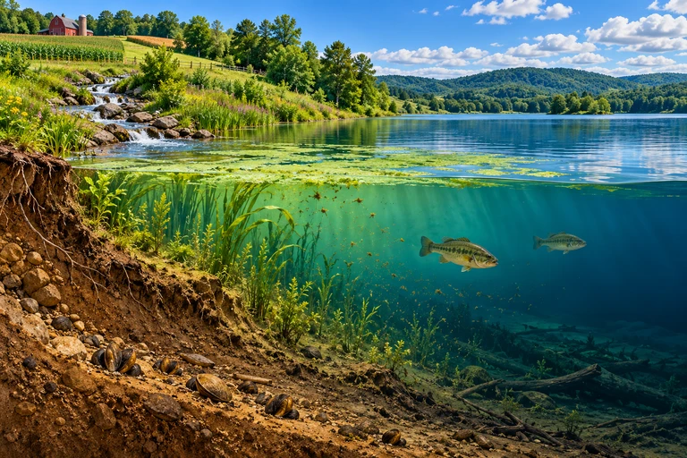A farm stream enters a cutaway lake with a partial green surface bloom, settling brown flecks, living fish in upper water and mussels near the bottom. Nutrient enrichment can increase algal production. Sinking organic matter fuels aerobic decomposer respiration, which consumes dissolved oxygen; restricted mixing can worsen bottom-water hypoxia.

Respiration links a bloom to low O₂. Nutrient enrichment can increase algal production. Sinking organic matter fuels aerobic decomposer respiration, which consumes dissolved oxygen; restricted mixing can worsen bottom-water hypoxia. 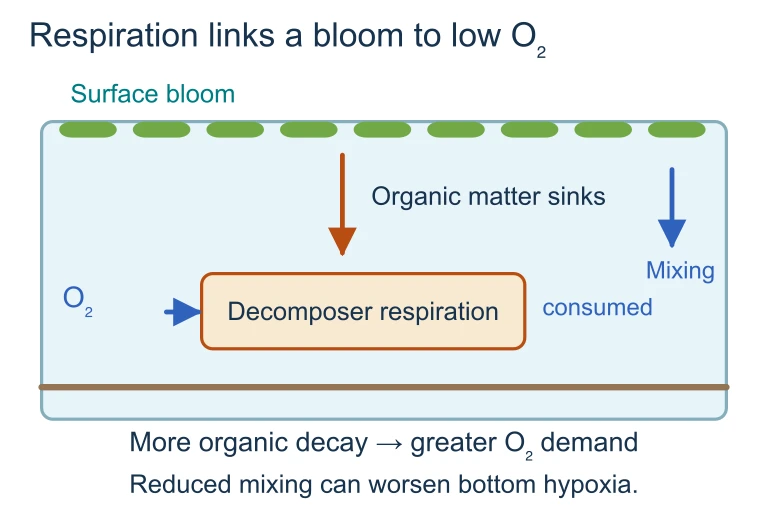Nutrient enrichment can increase algal production. Sinking organic matter fuels aerobic decomposer respiration, which consumes dissolved oxygen; restricted mixing can worsen bottom-water hypoxia.

SECTION 7

Natural vs. Anthropogenic Disruptions

A common AP Biology question type asks students to compare and contrast natural and human-caused disruptions. While both can profoundly alter ecosystems, they differ in several key dimensions that influence whether and how quickly recovery occurs.

Dimension	Natural Disruptions	Anthropogenic Disruptions
Evolutionary history	Species have often evolved adaptations to recurring natural disturbances (e.g., fire-dependent seed germination in chaparral)	Novel stressors (synthetic pesticides, microplastics) may not have any evolutionary analog, so species lack adaptive responses
Frequency & Predictability	Often periodic and somewhat predictable (seasonal floods, fire return intervals), allowing co-evolved community responses	May be continuous (pollution), sudden (oil spills), or accelerating (climate change), outpacing adaptive capacity
Spatial scale	Usually local to regional; surrounding intact habitat serves as a source for recolonization	Can be global (climate change, ozone depletion); fragmented landscapes limit dispersal corridors for recolonizers
Biological legacy	Often preserves soil, seed banks, and surviving organisms that accelerate secondary succession	May strip biological legacies entirely (e.g., mountaintop removal mining) or contaminate soil, hindering recovery
Synergistic effects	Typically operate independently or in well-characterized combinations	Multiple anthropogenic stressors interact unpredictably (e.g., warming + acidification + overfishing on coral reefs)

Key differences between natural and anthropogenic ecosystem disruptions

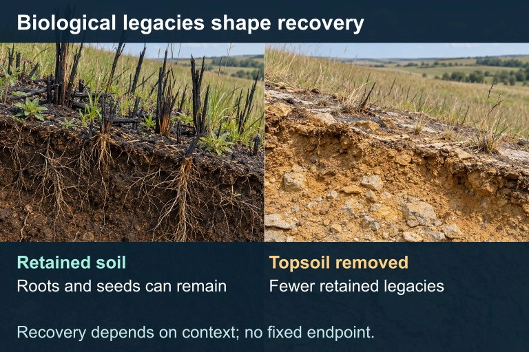Retained soil can preserve roots and a seed bank; removed topsoil leaves fewer biological legacies. Recovery depends on context.

SECTION 8

Regime Shifts & Ecological Thresholds

The most consequential outcome of ecosystem disruption is a regime shift—a rapid, often irreversible transition from one stable ecological state to another. Contemporary ecological theory frames this concept using alternative stable state models, in which an ecosystem can exist in multiple configurations (e.g., a clear-water lake with submerged vegetation versus a turbid, algae-dominated lake), and the transition between states is governed by critical thresholds. Once a threshold is crossed, positive feedback loops lock the system into the new state, making recovery difficult even if the original stressor is removed.

Concept	AP Biology Level	Advanced Ecological Theory
Succession	Linear sequence from pioneer to climax community; generally predictable	Multiple successional pathways; priority effects and stochastic assembly; climax concept largely abandoned
Resilience	Ability to return to original state after disturbance	Measured as the size of the 'basin of attraction'—how large a perturbation the system can absorb before shifting to an alternative state
Biodiversity–stability	Greater biodiversity generally increases ecosystem stability	Insurance hypothesis: functional redundancy among species buffers ecosystem processes; portfolio effect reduces variance in aggregate properties
Tipping points	Some disruptions cause permanent changes	Hysteresis: the path to degradation differs from the path to recovery, requiring greater remediation effort than the original disturbance magnitude

AP-level versus advanced ecological frameworks for understanding disruption

For the AP exam, you should be able to explain how human activities push ecosystems toward threshold transitions and why positive feedback loops make recovery nonlinear. A coral reef that loses its coral cover due to bleaching, for instance, is colonized by macroalgae that further inhibit coral recruitment, creating a feedback loop that maintains the degraded state even if water temperatures return to normal. Recognizing these dynamics connects the topic of ecosystem disruption to broader themes of homeostasis, feedback regulation, and the emergent properties of complex biological systems.

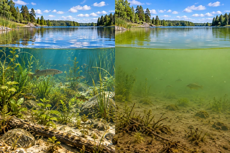Matched shallow basins show submerged vegetation in clearer water versus sparse vegetation and suspended material in turbid water. Scene alone does not establish persistence or alternative attractors. Separate exact panel: A signed feedback loop links submerged plants negatively to sediment resuspension, resuspension positively to turbidity and turbidity negatively to plants. Submerged plants reduce sediment resuspension; resuspension raises turbidity, and turbidity suppresses plant growth. This reinforcing loop can maintain a turbid shallow lake; evidence of hysteresis requires more than persistence alone.

A reinforcing shallow-lake loop. Submerged plants reduce sediment resuspension; resuspension raises turbidity, and turbidity suppresses plant growth. This reinforcing loop can maintain a turbid shallow lake; evidence of hysteresis requires more than persistence alone. 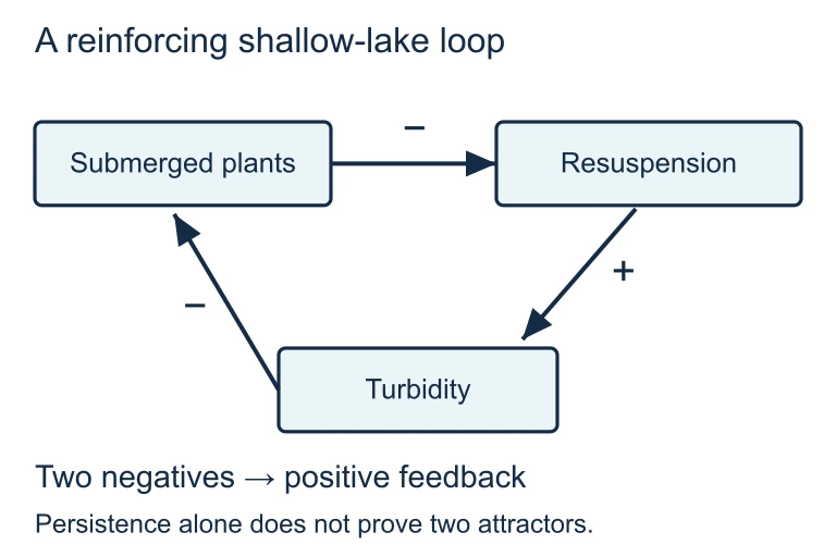Submerged plants reduce sediment resuspension; resuspension raises turbidity, and turbidity suppresses plant growth. This reinforcing loop can maintain a turbid shallow lake; evidence of hysteresis requires more than persistence alone.

SECTION 9

Practice Problems

Question 1: CONCEPTUAL

A forest ecosystem experiences a severe wildfire that destroys all above-ground vegetation but leaves the soil and root systems intact. Which of the following best describes the recovery process that will follow?

A. Primary succession, beginning with lichens colonizing bare rock
B. Secondary succession, beginning with fast-growing herbaceous species exploiting intact soil and seed banks
C. A permanent regime shift to grassland because the climax tree species were eliminated
D. No succession, because the disturbance exceeded the ecosystem's resistance threshold

Show answer (B)

B is correct. Secondary succession occurs when biological legacies (soil, seed banks, root systems, surviving organisms) remain after a disturbance, allowing relatively rapid recolonization by herbaceous pioneer species followed by shrubs and eventually trees. A is incorrect because primary succession requires bare substrate devoid of soil, which is not the case here since soil and roots are intact. C is incorrect because many tree species have fire-adapted traits (e.g., serotinous cones, fire-stimulated seed germination) and the presence of intact soil makes forest recovery likely, though species composition may shift. D is incorrect because succession occurs after virtually any disturbance—the ecosystem will reorganize, even if the trajectory differs from the pre-disturbance state.

Question 2: BASIC CALCULATION

In a marine food chain, phytoplankton (producers) fix 10,000 kcal/m²/year of energy. If trophic efficiency is 10% at each transfer, and a pollutant disrupts phytoplankton productivity by 40%, approximately how much energy (kcal/m²/year) would be available to tertiary consumers in the disrupted ecosystem?

A. 0.6 kcal/m²/year
B. 6.0 kcal/m²/year
C. 10 kcal/m²/year
D. 60 kcal/m²/year

Show answer (B)

B is correct. First, calculate the disrupted producer energy: 10,000 × 0.60 = 6,000 kcal/m²/year. In standard AP Biology terminology, tertiary consumers occupy the fourth trophic level (TL4): producers (TL1) → primary consumers (TL2) → secondary consumers (TL3) → tertiary consumers (TL4). This means there are three energy transfers from producers to tertiary consumers, each at 10% efficiency. Therefore: 6,000 × (0.10)³ = 6,000 × 0.001 = 6.0 kcal/m²/year. Choice A (0.6 kcal/m²/year) is incorrect because it applies four energy transfers (0.10⁴), which would correspond to quaternary consumers at TL5, not tertiary consumers at TL4. Choice C (10 kcal/m²/year) represents the energy available to tertiary consumers in the undisrupted ecosystem: 10,000 × (0.10)³ = 10 kcal/m²/year. This fails to account for the 40% reduction in producer productivity. Choice D (60 kcal/m²/year) represents the disrupted energy available to secondary consumers (TL3), not tertiary consumers: 6,000 × (0.10)² = 60 kcal/m²/year. The 40% loss at the producer level cascades proportionally through the entire food chain, reducing tertiary consumer energy from 10 to 6.0 kcal/m²/year.

Question 3: INTERMEDIATE

In a lake ecosystem, researchers observed that after the introduction of an invasive fish species, the population of native zooplankton declined by 80%, phytoplankton density increased dramatically, and water clarity decreased. Which of the following best explains the mechanism driving this set of observations?

A. The invasive fish out-competed phytoplankton for dissolved nutrients, altering light penetration
B. The invasive fish preyed on zooplankton, releasing phytoplankton from grazing pressure in a top-down trophic cascade
C. The invasive fish introduced a novel pathogen that selectively killed zooplankton through direct transmission
D. The invasive fish increased nutrient cycling by consuming benthic detritus, causing bottom-up eutrophication

Show answer (B)

B is correct. This is a classic top-down trophic cascade. The invasive fish preys heavily on zooplankton (primary consumers), reducing zooplankton grazing on phytoplankton (producers). Released from herbivory, phytoplankton populations bloom, increasing turbidity and reducing water clarity. A is incorrect because fish do not compete with phytoplankton for dissolved nutrients—they occupy entirely different trophic levels. C is not the best explanation because while pathogen introduction is possible, the correlated increase in phytoplankton and decrease in water clarity are most parsimoniously explained by reduced grazing, not disease. D describes a bottom-up mechanism, but the observations (zooplankton decline, phytoplankton increase) are most consistent with a top-down cascade where predation on zooplankton releases phytoplankton; bottom-up eutrophication would increase both zooplankton and phytoplankton rather than decreasing zooplankton.

Question 4: APPLIED

4 pts

A team of ecologists hypothesizes that the introduction of the invasive plant species purple loosestrife (Lythrum salicaria) into a temperate wetland reduces native plant species diversity by outcompeting them for light and space. Design a controlled field experiment to test this hypothesis. In your response: (a) Identify the independent variable, dependent variable, and at least two controlled variables. (b) Describe the experimental setup, including the control group and treatment group. (c) Predict the expected results if the hypothesis is supported, and describe what data you would collect. (d) Identify one potential confounding variable and explain how you would address it.

Show answer

Rubric (4 points): Point 1 — Variables (1 pt): Independent variable: presence/absence (or density) of purple loosestrife. Dependent variable: native plant species diversity (measured as species richness and/or Shannon diversity index). Controlled variables: plot size, soil type, hydrology/water level, initial native plant community composition, and sunlight exposure. Award 1 point for correctly identifying all three variable types with at least two controlled variables. Point 2 — Experimental design (1 pt): Establish multiple paired plots within the wetland. Control plots: native plant communities with no purple loosestrife (remove any that colonize). Treatment plots: native plant communities with purple loosestrife introduced at a standardized density. Include replication (e.g., ≥10 plots per treatment) and random assignment of plots to treatment/control. Award 1 point for a design that includes a control group, a treatment group, replication, and random assignment. Point 3 — Predicted results and data collection (1 pt): If the hypothesis is supported, treatment plots will show significantly lower native plant species richness and/or diversity index values compared to control plots over the experimental period (e.g., 1–3 growing seasons). Data collection: conduct periodic vegetation surveys using quadrats to count species identity and percent cover of each species. Statistical comparison (e.g., t-test or ANOVA) of mean diversity between groups. Award 1 point for a prediction consistent with the hypothesis and appropriate data collection methods. Point 4 — Confounding variable (1 pt): A potential confounding variable is variation in soil nutrient levels across plots, which could independently affect plant growth and diversity. This can be addressed by measuring baseline soil nutrient concentrations in all plots before the experiment begins and either stratifying plot assignment by nutrient levels or including soil nutrients as a covariate in statistical analysis. Other acceptable confounding variables include herbivore activity, microclimate variation, or seed dispersal from adjacent areas. Award 1 point for identifying a plausible confound and describing a method to control or account for it.

Question 5: CRITICAL THINKING

4 pts

Researchers studied the effects of coral bleaching on a tropical reef ecosystem over 10 years. The data below were collected at three time points. Year 0 (pre-bleaching): Coral cover = 60%, macroalgae cover = 5%, herbivorous fish biomass = 200 kg/hectare, species richness = 150 species. Year 3 (post-bleaching event): Coral cover = 15%, macroalgae cover = 40%, herbivorous fish biomass = 180 kg/hectare, species richness = 95 species. Year 10: Coral cover = 12%, macroalgae cover = 55%, herbivorous fish biomass = 80 kg/hectare, species richness = 60 species. (a) Describe the trends in coral cover and macroalgae cover from Year 0 to Year 10. Explain the biological mechanism responsible for the observed shift in cover between these two groups. (b) Explain why herbivorous fish biomass declined between Year 3 and Year 10 despite the increase in macroalgae, which serves as their food source. (c) Using the concept of alternative stable states, explain why coral cover continued to decline between Year 3 and Year 10 even though the initial bleaching event occurred between Year 0 and Year 3. (d) Propose one management intervention that could promote reef recovery, and explain its ecological rationale by referencing a specific mechanism in the feedback loop described in part (c).

Show answer

Rubric (4 points): Point 1 — Trend description and mechanism (1 pt): Coral cover declined sharply from 60% to 15% after the bleaching event and continued declining to 12% by Year 10, while macroalgae cover increased from 5% to 55%. The mechanism: thermal stress caused corals to expel their endosymbiotic zooxanthellae (dinoflagellates of genus Symbiodinium), depriving corals of their primary energy source via photosynthesis. Dead coral substrate was then colonized by fast-growing macroalgae, which outcompeted coral recruits for space and light. Award 1 point for describing the inverse trends and correctly explaining the bleaching, zooxanthellae expulsion, and algal colonization mechanism. Point 2 — Herbivorous fish decline (1 pt): Although macroalgae increased, herbivorous fish biomass declined because coral reefs provide critical three-dimensional habitat structure (shelter, breeding sites, refuge from predation). As coral cover declined, the loss of structural complexity reduced the carrying capacity for reef fish, including herbivores. Additionally, declining species richness suggests broader ecosystem degradation that may include loss of fish recruitment, increased predation in simplified habitats, or reduced overall productivity. The key insight is that food availability alone does not determine population size — habitat structure is equally critical. Award 1 point for connecting fish decline to loss of reef structural complexity rather than food limitation. Point 3 — Alternative stable states (1 pt): The continued decline of coral cover after the initial bleaching event illustrates a positive feedback loop characteristic of alternative stable states. Once macroalgae colonize dead coral, they inhibit coral larval settlement and recruitment through physical overgrowth, shading, and chemical allelopathy. Meanwhile, declining herbivorous fish populations reduce grazing pressure on macroalgae, further reinforcing algal dominance. The system has crossed a critical threshold into a macroalgae-dominated stable state, and hysteresis means that simply removing the initial stressor (thermal stress) is insufficient to restore coral dominance. Award 1 point for invoking positive feedback and explaining why the degraded state persists beyond the original disturbance. Point 4 — Management intervention (1 pt): Establishing marine protected areas (MPAs) that prohibit fishing of herbivorous fish species would allow herbivore populations to recover, increasing grazing pressure on macroalgae and creating open substrate for coral recruitment. This breaks the positive feedback loop by restoring top-down control of algae. Other acceptable answers include: active coral reef restoration (transplanting coral fragments), reducing land-based nutrient pollution to limit algal growth (bottom-up control), or assisted gene flow of heat-tolerant coral genotypes. Award 1 point for a biologically justified intervention that targets a specific mechanism in the feedback loop.