Community Ecology - AP Biology

SECTION 1

Historical Context & Motivation

Ecology as a formal discipline emerged in the late nineteenth century, but the study of how species coexist and interact within shared habitats traces back much further. Early naturalists such as Alexander von Humboldt recognized that organisms do not exist in isolation—their distributions and abundances are shaped by the web of relationships they maintain with other species. The central question of community ecology is deceptively simple: why do certain species live together, and what determines how many species a given habitat can support? Answering this question required breakthroughs in understanding competition, predation, mutualism, and disturbance—each contributing a piece to the ecological puzzle. The intellectual arc from early observational natural history to rigorous experimental ecology illuminates how our modern understanding of biological communities was assembled.

1934 • Gause's Competitive Exclusion Principle

G.F. Gause demonstrated through laboratory experiments with Paramecium species that two species competing for identical resources cannot stably coexist—one will inevitably outcompete the other.

1958 • Hutchinson's Niche Concept

G. Evelyn Hutchinson formalized the n-dimensional hypervolume niche concept, distinguishing the fundamental niche (all conditions a species can tolerate) from the realized niche (what it actually occupies due to interactions).

1966 • Paine's Keystone Species

Robert Paine's experimental removal of the sea star Pisaster ochraceus from intertidal communities revealed that a single predator could disproportionately maintain species diversity, coining the term keystone species.

1967 • MacArthur & Wilson's Island Biogeography

Robert MacArthur and E.O. Wilson published their equilibrium theory of island biogeography, modeling species richness as a balance between immigration and extinction rates—a framework still central to conservation biology.

1978 • Connell's Intermediate Disturbance Hypothesis

Joseph Connell proposed that moderate levels of disturbance promote the highest species diversity in communities, preventing competitive exclusion without eliminating most species.

These milestones collectively frame the central challenge of community ecology: how do interspecific interactions, environmental conditions, and stochastic events combine to produce the patterns of biodiversity we observe? The AP Biology curriculum expects you to evaluate these mechanisms both qualitatively and through data analysis, making this topic one of the most integrative in the course.

SECTION 2

Core Principles & Definitions

A biological community consists of all the populations of different species that live and interact within a particular area at a given time. Community ecology examines the structure of these assemblages—measured by species richness (the number of species present), relative abundance (the proportion of each species), and species diversity (which combines both richness and evenness). The interactions among species, the physical environment, and evolutionary history all shape these parameters. Understanding the following core principles provides the conceptual toolkit for analyzing any community.

Interspecific Interactions

Species relationships—competition (−/−), predation (+/−), mutualism (+/+), commensalism (+/0), and parasitism (+/−)—are the engines that drive community structure and determine which species persist.

Competitive Exclusion & Niche Partitioning

Two species occupying the same ecological niche cannot coexist indefinitely. Coexistence requires resource partitioning—dividing the niche along spatial, temporal, or dietary axes so that each species exploits slightly different resources.

Trophic Structure

Communities are organized into feeding levels: producers, primary consumers, secondary consumers, and decomposers. Energy flow and nutrient cycling through these levels constrain community biomass and diversity.

Keystone Species & Dominant Species

A keystone species exerts influence far exceeding its biomass (e.g., a top predator preventing competitive exclusion), while a dominant species controls community dynamics through sheer abundance and resource capture.

Ecological Succession

Communities change over time through primary succession (colonizing bare substrate) or secondary succession (recovery after disturbance). Pioneer species give way to later-successional species, potentially reaching a climax community.

✦

KEY TAKEAWAY

Think of a biological community like an orchestra. Each species is an instrument with a unique role (its ecological niche). If two violinists try to play the exact same part, one will be drowned out (competitive exclusion). But when each instrument plays a different part, the ensemble produces a richer, more resilient performance—just as niche partitioning promotes greater species diversity and community stability.

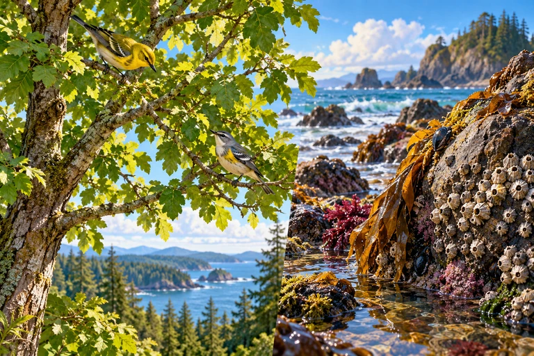
Two foraging birds in different portions of a tree, beside a separate rocky barnacle shore. Resource partitioning reduces overlap in resource use. A separate competitor-removal comparison tests whether competition limits a species’ realized distribution on the shore.

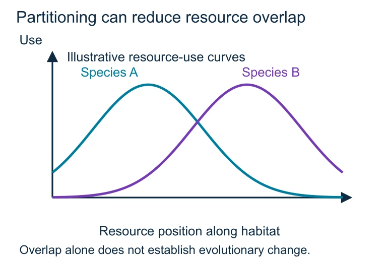
Partitioning can reduce resource overlap. Resource partitioning reduces overlap in resource use. A separate competitor-removal comparison tests whether competition limits a species’ realized distribution on the shore. Resource partitioning reduces overlap in resource use. A separate competitor-removal comparison tests whether competition limits a species’ realized distribution on the shore.

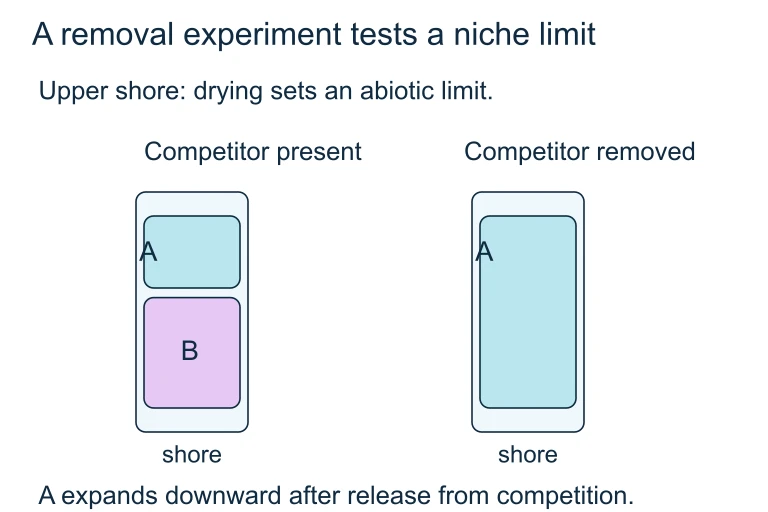
A removal experiment tests a niche limit. Removing a competitor allows a shore species to expand downward while its upper drying limit persists, distinguishing biotic and abiotic limits. Removing a competitor allows a shore species to expand downward while its upper drying limit persists, distinguishing biotic and abiotic limits.

SECTION 3

Interspecific Interactions — Visual Overview

The five major categories of interspecific interactions, classified by their effects on each species involved. The +/− notation indicates whether a species benefits (+), is harmed (−), or is unaffected (0).

The diagram above summarizes the five fundamental categories of species interactions that the AP Biology exam expects you to distinguish. Notice that predation and parasitism share the same +/− notation, yet they differ in mechanism: a predator typically kills its prey outright, whereas a parasite exploits a living host over an extended period. Similarly, competition can be exploitative (both species deplete the same resource) or interference (one species directly prevents the other from accessing the resource). These subtleties often appear in AP free-response questions, where you must identify the interaction type from experimental data and justify your reasoning with evidence.

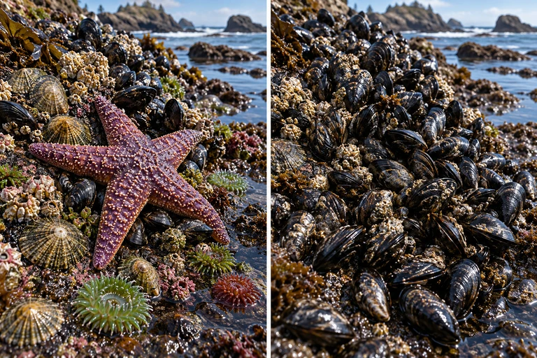
Foreground sea star has five arms; left rock contains several sessile forms while right is mussel dominated. Composition is a conceptual comparison, not historical data. Separate exact panel: Two negative causal links connect sea stars to mussels and mussels to other sessile taxa, yielding a positive indirect effect on other taxa. Sea-star predation can reduce mussel dominance and indirectly release other sessile species from competition. A removal experiment compares treated and control plots through time.

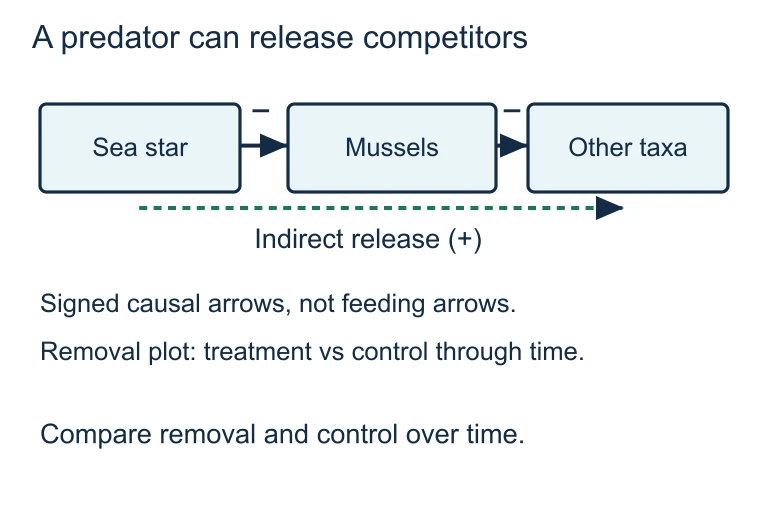
A predator can release competitors. Sea-star predation can reduce mussel dominance and indirectly release other sessile species from competition. A removal experiment compares treated and control plots through time. Sea-star predation can reduce mussel dominance and indirectly release other sessile species from competition. A removal experiment compares treated and control plots through time.

SECTION 4

Quantifying Diversity — The Mathematical Framework

While much of community ecology is qualitative, several quantitative tools allow ecologists to compare communities rigorously. The AP Biology exam focuses on species diversity indices, which incorporate both species richness and evenness into a single metric. A community with many species distributed equally is more diverse than one dominated by a single species. Understanding these indices allows you to interpret ecological data sets and evaluate claims about habitat quality or conservation priorities.

SHANNON DIVERSITY INDEX

H = −Σ (pᵢ × ln pᵢ)

H = Shannon diversity index; pᵢ = proportion of individuals belonging to the iᵗʰ species; ln = natural logarithm; Σ = summation over all species. Higher H values indicate greater diversity.

SIMPSON'S DIVERSITY INDEX

D = 1 − Σ (pᵢ²)

D = Simpson's diversity index; pᵢ = proportion of individuals belonging to the iᵗʰ species. D ranges from 0 (no diversity) to nearly 1 (high diversity). This index emphasizes dominance—it represents the probability that two randomly selected individuals belong to different species.

SPECIES RICHNESS VS. EVENNESS

Diversity = f(Richness, Evenness)

Species richness (S) = total number of species. Evenness (E) = how equally individuals are distributed among species. Two communities can have the same S but very different diversity if their evenness differs. On the AP exam, you may be asked to compare communities using both metrics.

💡

AP EXAM TIP

You are not required to memorize the Shannon or Simpson formulas for the AP Biology exam, but you must be able to interpret calculated diversity values, compare communities, and explain how changes in richness or evenness affect diversity. Practice reading data tables and calculating proportions.

SECTION 5

Ecological Succession — Community Change Over Time

Communities are not static—they change predictably through a process called ecological succession. Primary succession occurs on newly exposed substrates devoid of soil, such as cooled lava flows or retreating glaciers, where pioneer species like lichens and mosses initiate soil formation. Secondary succession occurs after a disturbance (fire, logging, hurricane) removes most existing vegetation but leaves the soil intact, allowing faster recovery. In both cases, early-successional species are typically r-selected (rapid reproduction, high dispersal) and are gradually replaced by K-selected species (slower growth, superior competitive ability) as the community matures. The endpoint—sometimes called a climax community—remains relatively stable unless disturbed, though ecologists increasingly recognize that most communities exist in a state of dynamic equilibrium rather than a fixed endpoint.

Primary succession from bare rock to climax forest. The solid green line represents total community biomass accumulation over time; the dashed cyan line represents species diversity, which initially rises steeply, then plateaus or may slightly decline as dominant competitors exclude some pioneer species.

As shown in the diagram, species diversity does not increase without limit during succession. The intermediate disturbance hypothesis, proposed by Connell, explains this pattern: at low disturbance frequency, competitive dominants exclude other species, reducing diversity; at high disturbance frequency, only disturbance-tolerant species survive. Maximal diversity occurs at intermediate disturbance levels, where both early- and late-successional species coexist. This concept frequently appears on the AP exam in the context of data interpretation questions about disturbance regimes and their effects on biodiversity.

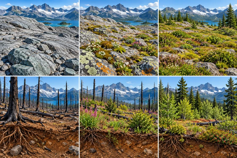
Two rows compare bare glacial rock becoming vegetated with burned woodland recovering above visible retained soil and roots; later patches contain mixed open vegetation and trees. Primary succession begins without developed soil; secondary succession retains soil and biological legacies. Climate, dispersal and later disturbance influence recovery and the communities that develop.

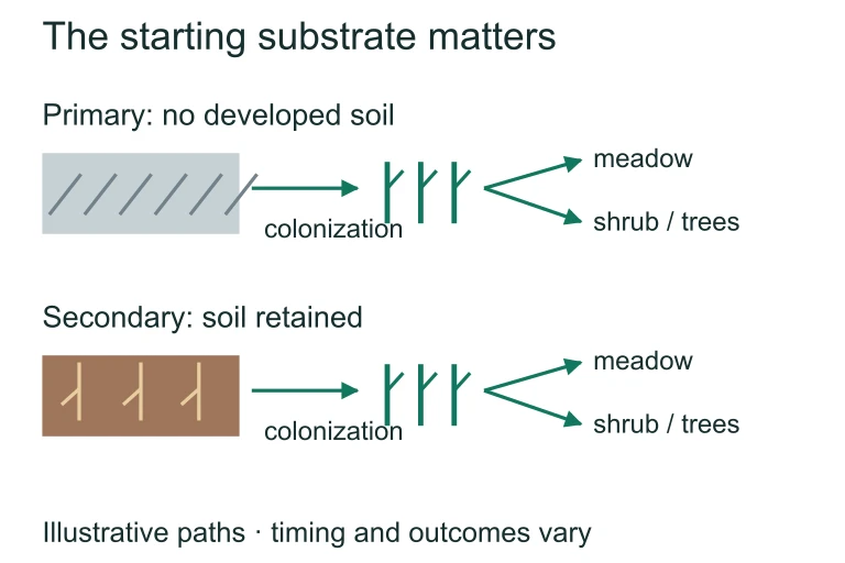
The starting substrate matters. Primary succession begins without developed soil; secondary succession retains soil and biological legacies. Climate, dispersal and later disturbance influence recovery and the communities that develop. Primary succession begins without developed soil; secondary succession retains soil and biological legacies. Climate, dispersal and later disturbance influence recovery and the communities that develop.

SECTION 6

Worked Example — Calculating Simpson's Diversity Index

Consider two pond communities, each containing 100 individuals. Pond A has 4 species with abundances of 25, 25, 25, and 25 individuals. Pond B has 4 species with abundances of 85, 5, 5, and 5 individuals. Which pond is more diverse according to Simpson's Diversity Index?

Comparing Pond Diversity Using Simpson's Index

1
Step 1 — Calculate Proportions (pᵢ) for Each Pond

For Pond A, each species contributes 25/100 = 0.25 of the total community. For Pond B, the proportions are: Species 1 = 85/100 = 0.85, Species 2 = 5/100 = 0.05, Species 3 = 0.05, Species 4 = 0.05.

Pond A: pᵢ = {0.25, 0.25, 0.25, 0.25}; Pond B: pᵢ = {0.85, 0.05, 0.05, 0.05}
2
Step 2 — Square Each Proportion

For Pond A: (0.25)² = 0.0625 for each of 4 species. For Pond B: (0.85)² = 0.7225, (0.05)² = 0.0025 for each of the remaining 3 species.

Pond A squares: {0.0625, 0.0625, 0.0625, 0.0625}; Pond B squares: {0.7225, 0.0025, 0.0025, 0.0025}
3
Step 3 — Sum the Squared Proportions (Σ pᵢ²)

For Pond A: 4 × 0.0625 = 0.25. For Pond B: 0.7225 + 3 × 0.0025 = 0.7225 + 0.0075 = 0.73.

Σ pᵢ² Pond A = 0.25; Σ pᵢ² Pond B = 0.73
4
Step 4 — Apply Simpson's Formula: D = 1 − Σ pᵢ²

Pond A: D = 1 − 0.25 = 0.75. Pond B: D = 1 − 0.73 = 0.27.

Pond A: D = 0.75; Pond B: D = 0.27
5
Step 5 — Interpret the Result

Although both ponds have the same species richness (S = 4), Pond A has dramatically higher diversity (D = 0.75 vs. 0.27). This difference reflects evenness: Pond A's individuals are distributed equally among species, while Pond B is dominated by a single species. This example illustrates a core AP Biology principle—species richness alone does not capture the full picture of community diversity.

Pond A is more diverse due to higher evenness, despite equal species richness.

SECTION 7

Comparing Species Interactions — Ecological Effects

Interaction Type	Effect on Community Structure	Example & AP Relevance
Competition	Limits coexistence; drives niche partitioning or local extinction of the weaker competitor. Reduces realized niche breadth.	Gause's Paramecium experiments; Connell's barnacle studies (frequently tested).
Predation	Controls prey populations; can increase diversity by preventing competitive exclusion (keystone predation). Drives evolutionary arms races.	Paine's sea star removal; lynx-hare population cycles. AP FRQs often present predator-prey data.
Mutualism	Facilitates community productivity and enables species to exploit niches they otherwise could not. Can be obligate or facultative.	Mycorrhizal fungi and plants; coral and zooxanthellae. Key for understanding reef and forest ecosystems.
Parasitism	Weakens host fitness; can regulate host populations similar to predation. Coevolutionary dynamics shape host immune responses.	Plasmodium (malaria) and mosquito-human cycle; nematode infections in wildlife.
Commensalism	One species benefits without measurably affecting the other. Difficult to confirm because subtle costs/benefits may exist.	Epiphytic orchids on tropical trees; cattle egrets following herds.

Comparison of interspecific interactions and their roles in structuring communities.

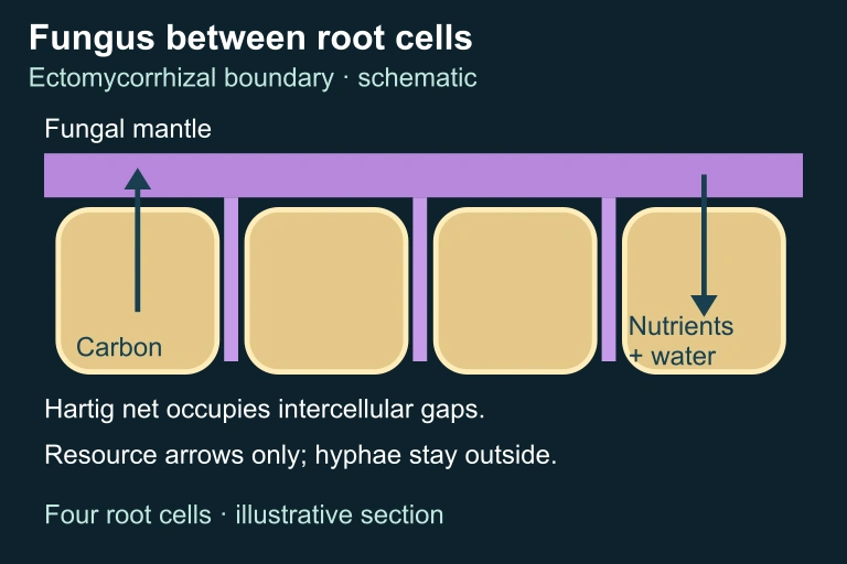
Ectomycorrhizal boundary

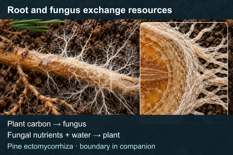
Root and fungal threads illustrate pine ectomycorrhiza. Plant carbon moves to the fungus and nutrients and water move to the plant. A companion depicts four root cells and a Hartig net in intercellular gaps. In a generic pine ectomycorrhiza, fungal hyphae surround the root and extend between outer root cells. Plant carbon moves toward the fungus while nutrients and water can move toward the plant; benefits depend on conditions.

✦

KEY TAKEAWAY

Species interactions function like the checks and balances in a political system. Competition limits monopolies, predation prevents any single population from dominating, and mutualism creates cooperative alliances that strengthen the whole. When a keystone interaction is removed—like removing the judiciary from government—the entire structure can destabilize, often with a dramatic loss of diversity.

SECTION 8

From Community Ecology to Ecosystem & Global Ecology

Community ecology sits at a pivotal position in the hierarchy of biological organization. Below it, population ecology examines single-species dynamics; above it, ecosystem ecology integrates the biotic community with the abiotic environment to trace energy flow and nutrient cycling. Many AP Biology questions bridge these levels, asking how a change in community composition (such as loss of a keystone species) cascades into ecosystem-level consequences like altered primary productivity or disrupted biogeochemical cycles. Understanding this connectivity is essential for tackling interdisciplinary free-response questions.

Feature	Community Ecology	Ecosystem Ecology
Focus	Species interactions, diversity, and composition	Energy flow, nutrient cycling, and productivity
Components	Biotic only (all populations in an area)	Biotic + abiotic (community plus physical environment)
Key Metrics	Species richness, diversity indices, relative abundance	GPP, NPP, trophic efficiency, decomposition rate
Example Question	How does removing a predator affect prey species diversity?	How does removing a predator alter carbon cycling in the ecosystem?
Evolutionary Link	Coevolution, character displacement, mimicry	Biogeochemical adaptations, global climate feedbacks

Comparing community ecology and ecosystem ecology — how the scope of analysis shifts.

Looking forward, concepts from community ecology directly inform conservation biology and global change biology. The theory of island biogeography, for example, is applied to habitat fragments treated as ecological "islands" surrounded by inhospitable terrain. Conservation corridors, reserve design, and predictions about extinction debt all draw on the same principles of immigration, extinction, and species-area relationships that MacArthur and Wilson formalized for oceanic islands. As you move into AP Environmental Science or college-level ecology courses, these community-level principles will expand into landscape ecology and macroecology.

SECTION 9

Practice Problems

Question 1: CONCEPTUAL

A marine biologist removes a top predator species from an intertidal community and observes that one mussel species rapidly outcompetes all other sessile invertebrates, reducing overall species diversity. The removed predator is best described as which of the following?

A. A dominant species, because it was the most abundant organism in the community
B. An invasive species, because its removal allowed a native species to expand
C. A keystone species, because its removal caused a disproportionate change in community structure relative to its abundance
D. A pioneer species, because it was the first to colonize the intertidal zone

Show answer (C)

C is correct. A keystone species exerts an influence on community structure that is disproportionately large relative to its biomass or abundance. This scenario directly mirrors Robert Paine's classic experiment with Pisaster ochraceus, where removing the predatory sea star allowed mussels to dominate and exclude other species. A is incorrect because the question describes the predator, not the mussel, and dominance refers to abundance and resource capture, not to the predator's regulatory role. B is incorrect because nothing in the scenario indicates the predator was non-native; invasive species status depends on origin, not ecological effect. D is incorrect because pioneer species are early colonizers in succession, which is unrelated to the predator's role described here.

Question 2: BASIC CALCULATION

A researcher surveys two meadow plots, each containing 200 individual organisms. Plot X has 5 species with 40 individuals each. Plot Y has 5 species with abundances of 160, 10, 10, 10, and 10. Using Simpson's Diversity Index (D = 1 − Σpᵢ²), which of the following correctly compares the two plots?

A. Plot X: D = 0.80; Plot Y: D = 0.36
B. Plot X: D = 0.20; Plot Y: D = 0.64
C. Plot X: D = 0.80; Plot Y: D = 0.80
D. Plot X: D = 0.50; Plot Y: D = 0.36

Show answer (A)

A is correct. For Plot X: each pᵢ = 40/200 = 0.20, so pᵢ² = 0.04, and Σpᵢ² = 5 × 0.04 = 0.20; D = 1 − 0.20 = 0.80. For Plot Y: p₁ = 160/200 = 0.80, p₂ through p₅ = 10/200 = 0.05 each. Σpᵢ² = (0.80)² + 4 × (0.05)² = 0.64 + 0.01 = 0.65; D = 1 − 0.65 ≈ 0.36 (rounding). B is incorrect because it confuses D with Σpᵢ² (the values are inverted). C is incorrect because plots with different evenness cannot have the same diversity index despite equal richness. D is incorrect because the calculation for Plot X yields 0.80, not 0.50.

Question 3: INTERMEDIATE

Two closely related species of warblers coexist in the same forest. Species A forages primarily in the upper canopy, while Species B forages in the lower branches and understory. This pattern is best explained by which of the following ecological concepts?

A. Primary succession, because the species colonized different vertical zones at different times
B. Resource partitioning, because natural selection has favored divergence in foraging niches to reduce interspecific competition
C. Competitive exclusion, because one species has eliminated the other from its preferred zone
D. Mutualism, because both species benefit from occupying different parts of the tree

Show answer (B)

B is correct. This scenario describes resource partitioning (also called niche differentiation), the classic pattern documented by Robert MacArthur in his study of five warbler species in New England spruce forests. Each species reduces overlap by foraging in different parts of the tree, thereby permitting coexistence despite shared resources. A is incorrect because succession describes temporal community change on a landscape, not spatial foraging behavior. C is incorrect because both species still coexist—exclusion has not occurred; rather, competition has been reduced through niche divergence. D is incorrect because there is no mutual benefit exchange; the species are merely avoiding competition, which is not the same as a mutualistic interaction.

Question 4: APPLIED

4 pts

An ecologist hypothesizes that the sea otter (Enhydra lutris) functions as a keystone species in Pacific kelp forest ecosystems by controlling sea urchin populations, which would otherwise overgraze kelp. Design a field experiment to test this hypothesis. In your response: (a) State the null hypothesis. (b) Describe the experimental setup, including controls, treatments, and variables. (c) Explain what data should be collected and how they would support or refute the hypothesis. (d) Identify one potential confounding variable and describe how the experimental design accounts for it.

Show answer

Rubric — 4 points total: (a) Null hypothesis (1 point): The presence or absence of sea otters has no significant effect on sea urchin density or kelp forest cover in the experimental plots. Award 1 point for a correctly stated null hypothesis that references both the independent variable (otter presence) and at least one dependent variable (urchin density or kelp cover). (b) Experimental design (1 point): Identify multiple paired kelp forest sites of similar size, depth, wave exposure, and initial kelp density. Treatment sites: use exclusion cages or fencing to prevent sea otter access (or compare naturally otter-free vs. otter-present areas if exclusion cages are impractical). Control sites: matched plots where sea otters have normal access. The independent variable is sea otter presence/absence; dependent variables include sea urchin density, kelp canopy cover, and species diversity. Multiple replicates should be established to allow statistical analysis. Award 1 point for a design that includes appropriate controls, replication, and correctly identified independent and dependent variables. (c) Data collection and interpretation (1 point): At regular intervals (e.g., monthly over 1–2 years), measure sea urchin density per m², percent kelp canopy cover, and total species richness of invertebrates and fish within each plot. If otter-excluded plots show significantly higher urchin density, lower kelp cover, and reduced species diversity compared to controls, this supports the keystone hypothesis. If there is no significant difference, the null hypothesis is not rejected. Award 1 point for describing quantitative data collection methods and explicitly linking outcomes to accepting or rejecting the hypothesis. (d) Confounding variable (1 point): A potential confound is variation in water temperature, nutrient levels, or wave exposure between sites, which could independently affect kelp growth. This is controlled by selecting paired sites with similar physical conditions and by using multiple replicates across different locations to account for site-specific variation. Award 1 point for identifying a specific, plausible confounding variable and describing a reasonable strategy to mitigate it.

Question 5: CRITICAL THINKING

4 pts

A long-term study tracked species richness on three islands at different distances from a mainland source pool. The data are summarized below: • Island A (2 km from mainland): Initial species = 12; after 10 years = 30; after 50 years = 35 • Island B (15 km from mainland): Initial species = 8; after 10 years = 20; after 50 years = 22 • Island C (50 km from mainland): Initial species = 5; after 10 years = 12; after 50 years = 14 All three islands are approximately the same size. (a) Describe the overall trend observed in the data. (b) Explain this pattern using MacArthur and Wilson's equilibrium model of island biogeography. (c) Predict what would happen to the equilibrium species richness on Island A if the island's area were reduced by 50% due to rising sea levels. Justify your prediction. (d) A fourth island, Island D, is 15 km from the mainland but is four times larger than Island B. Predict how Island D's equilibrium species richness would compare to Island B's, and explain your reasoning.

Show answer

Rubric — 4 points total: (a) Trend description (1 point): All three islands showed increases in species richness over time, with richness rising rapidly in the first 10 years and then leveling off by 50 years, suggesting approach to an equilibrium. Islands closer to the mainland consistently supported more species than more distant islands of similar size. Award 1 point for describing both the temporal trend (rapid increase then plateau) and the distance-dependent pattern (near islands have more species). (b) Explanation using island biogeography (1 point): According to MacArthur and Wilson's model, species richness on an island reflects a dynamic equilibrium between immigration rate (new species arriving) and extinction rate (resident species disappearing). Islands closer to the mainland have higher immigration rates because dispersal is easier over shorter distances. Since all three islands are similar in size, their extinction rates should be comparable. Therefore, the equilibrium species number (where the immigration and extinction rate curves intersect) is higher for islands nearer the mainland. Award 1 point for correctly applying the equilibrium model with reference to immigration and extinction rate dynamics. (c) Prediction for reduced island area (1 point): If Island A's area were halved, the extinction rate would increase because smaller islands support smaller populations, which are more vulnerable to stochastic extinction events and have fewer available niches. The immigration rate would remain largely unchanged (distance to mainland is the same). Therefore, the new equilibrium point would shift to a lower species richness—the immigration and extinction curves would intersect at a lower value than the current ≈35 species. Award 1 point for predicting lower equilibrium richness and correctly reasoning that reduced area increases extinction rate while immigration rate is unaffected. (d) Prediction for Island D (1 point): Island D would have a higher equilibrium species richness than Island B. Both islands are equidistant from the mainland (15 km), so their immigration rates should be similar. However, Island D's larger area provides more habitat heterogeneity, supports larger populations, and therefore has a lower extinction rate. A lower extinction rate means the equilibrium intersection point shifts to a higher species number. This prediction is consistent with the species-area relationship, which holds that larger areas support more species. Award 1 point for the correct prediction (Island D > Island B) with reasoning that links larger area to lower extinction rate and higher equilibrium richness.

SUMMARY

Community Ecology — Summary

Summary

Community ecology examines how populations of different species interact within a shared environment and how those interactions shape species diversity, community composition, and ecological stability. The five major interspecific interactions—competition, predation, mutualism, commensalism, and parasitism—drive patterns of coexistence and exclusion. Competitive exclusion dictates that species occupying identical niches cannot coexist, leading to niche partitioning and character displacement as evolutionary responses.

Keystone species exert disproportionate control over community structure relative to their abundance, often by preventing competitive exclusion through predation. Ecological succession describes how communities change over time from pioneer stages through to climax communities, with diversity often peaking at intermediate levels of disturbance. Quantitative tools such as the Simpson's diversity index combine species richness and evenness to provide rigorous measures of community diversity. Finally, island biogeography theory models equilibrium species richness as a balance of immigration and extinction rates—a framework now widely applied in conservation biology to design nature reserves and predict biodiversity loss from habitat fragmentation.