
SECTION 1
Historical Context & Motivation
The concept of biodiversity—a contraction of "biological diversity"—was formalized only in the late twentieth century, but the intellectual roots stretch back to early naturalists who catalogued species across continents. Charles Darwin and Alfred Russel Wallace recognized that the sheer variety of organisms was both a product of evolution and a driver of ecological complexity. As industrialization accelerated habitat destruction, biologists grew increasingly alarmed that species were disappearing faster than they could be described. The term "biodiversity" was popularized during the 1986 National Forum on BioDiversity organized by E.O. Wilson, crystallizing decades of concern into a single unifying concept that now underpins conservation biology, ecosystem ecology, and environmental policy worldwide.
1735 • Linnaean Taxonomy
1859 • Origin of Species
1967 • Island Biogeography Theory
1986 • The BioDiversity Forum
1992 • Convention on Biological Diversity
The central question biodiversity science seeks to answer is deceptively simple: How many species exist, how are they distributed, and what happens to ecosystems when that variety declines? Answering this requires integrating genetics, taxonomy, ecology, and evolutionary biology—an interdisciplinary challenge at the heart of AP Biology's ecology unit.
SECTION 2
Core Principles & Definitions
Biodiversity is measured and discussed at three hierarchical levels, each capturing a different dimension of biological variation. These levels are interconnected: genetic diversity fuels species diversity through variation and selection, while species diversity contributes to the structural and functional complexity captured by ecosystem diversity. Understanding all three levels is essential for the AP Biology exam, which frequently tests the relationship between diversity at one level and stability or function at another.
Genetic Diversity
Species Diversity
Ecosystem Diversity
Species Richness vs. Evenness
SECTION 3
Visualizing Biodiversity Levels
The diagram above illustrates how biodiversity is structured across scales. At the smallest scale, genetic diversity is represented by the range of genotypes (AA, Aa, aa, etc.) within a single population—more alleles mean greater raw material for natural selection. At the community level, species diversity integrates both the count of species and their relative abundances, depicted by the bar chart's roughly equal heights. Finally, ecosystem diversity captures the breadth of distinct habitat types—forest, wetland, prairie—each supporting unique assemblages of species and ecological processes.
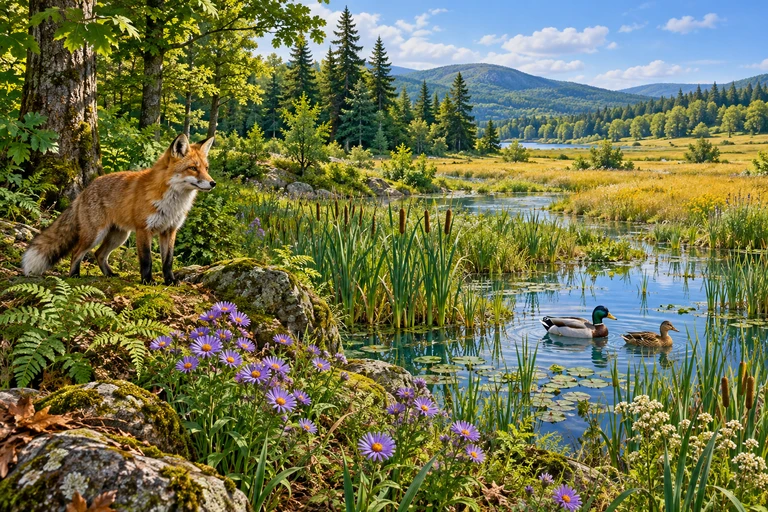 Biodiversity includes ecosystem variety across landscapes, species diversity within communities and genetic variation within a species. At one diploid two-allele locus, AA, Aa and aa are three genotypes formed from two alleles.
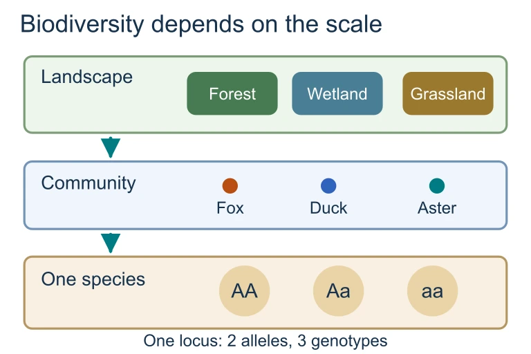 Biodiversity includes ecosystem variety across landscapes, species diversity within communities and genetic variation within a species. At one diploid two-allele locus, AA, Aa and aa are three genotypes formed from two alleles.
SECTION 4
Quantifying Biodiversity: Indices & Equations
Ecologists rely on mathematical indices to convert raw species-count data into comparable, interpretable measures of diversity. Two indices appear frequently on the AP Biology exam: the Shannon diversity index (H) and Simpson's diversity index (D). Both capture richness and evenness, but they differ in their mathematical emphasis: Shannon weighs rare species more heavily through the logarithm, while Simpson emphasizes the probability that two randomly selected individuals belong to different species.
SHANNON DIVERSITY INDEX
Where H = Shannon index value, pᵢ = proportion of total individuals belonging to species i, ln = natural logarithm, and the summation runs over all species in the community. Higher H indicates greater diversity.
SIMPSON'S DIVERSITY INDEX
Where D ranges from 0 to 1. A value near 1 indicates high diversity (low probability that two randomly chosen individuals are the same species), while a value near 0 indicates a community dominated by one species.
SPECIES-AREA RELATIONSHIP
Where S = number of species, A = area of habitat, c = y-intercept constant (varies by taxon/region), and z = slope of the species-area curve on a log-log plot (typically 0.1–0.35). This power-law relationship predicts species loss when habitat area is reduced.
SECTION 5
Threats to Biodiversity
Biodiversity loss is driven by a suite of interacting anthropogenic pressures often summarized by the acronym HIPPCO: Habitat destruction, Invasive species, Pollution, Population growth (human), Climate change, and Overexploitation. These threats do not operate in isolation; habitat fragmentation, for instance, reduces population sizes, which lowers genetic diversity, which in turn diminishes a species' capacity to adapt to climate change. Understanding the synergistic nature of these threats is essential for AP exam questions that ask you to evaluate conservation strategies.
Of these six drivers, habitat destruction is the single greatest threat to global biodiversity, responsible for the majority of recent species declines. Tropical deforestation alone eliminates an estimated 50,000–100,000 species per year (most undescribed invertebrates and fungi). The species-area relationship (S = cAz) predicts that a 90% reduction in habitat area can eliminate roughly 50% of species, assuming a typical z-value of 0.25. Climate change is projected to overtake habitat loss as the primary driver of extinction by mid-century, as shifting temperature and precipitation regimes outpace species' migration and adaptation capacities.
SECTION 6
Worked Example: Calculating Shannon Diversity Index
Suppose a field biologist surveys two forest communities and records the following species abundances. Community A has 4 species: 25, 25, 25, and 25 individuals respectively (total = 100). Community B has 4 species: 80, 10, 5, and 5 individuals (total = 100). Let's compute H for each community to determine which is more diverse.
Worked example
- 1
Step 1 — Calculate proportions (pᵢ)
Each species has 25 out of 100 individuals, so p₁ = p₂ = p₃ = p₄ = 25/100 = 0.25. - 2
Step 2 — Compute pᵢ × ln(pᵢ) for each species
For every species: 0.25 × ln(0.25) = 0.25 × (−1.386) = −0.347. Since all four species have the same proportion, each contributes −0.347. - 3
Step 3 — Sum and negate
Σ(pᵢ × ln pᵢ) = 4 × (−0.347) = −1.386. Therefore, H = −(−1.386).= 1.386
Worked example
- 1
Step 1 — Calculate proportions
p₁ = 80/100 = 0.80, p₂ = 10/100 = 0.10, p₃ = 5/100 = 0.05, p₄ = 5/100 = 0.05. - 2
Step 2 — Compute pᵢ × ln(pᵢ)
Species 1: 0.80 × ln(0.80) = 0.80 × (−0.223) = −0.178. Species 2: 0.10 × ln(0.10) = 0.10 × (−2.303) = −0.230. Species 3: 0.05 × ln(0.05) = 0.05 × (−2.996) = −0.150. Species 4: 0.05 × ln(0.05) = −0.150. - 3
Step 3 — Sum and negate
Σ = −0.178 + (−0.230) + (−0.150) + (−0.150) = −0.708. H = −(−0.708).= 0.708 - 4
Step 4 — Interpret
Community A (H = 1.386) is substantially more diverse than Community B (H = 0.708), even though both contain the same number of species (richness = 4). The difference is entirely due to evenness: Community A's equal abundances maximize H, while Community B's dominance by a single species depresses H.
SECTION 7
Biodiversity & Ecosystem Services
Biodiversity is not merely an aesthetic or ethical concern—it underpins the ecosystem services upon which human economies and well-being depend. These services are traditionally classified into four categories: provisioning, regulating, cultural, and supporting. Communities with higher species diversity tend to be more productive and more resistant to disturbance, a relationship known as the diversity-stability hypothesis. The AP exam may present data from biodiversity-manipulation experiments (e.g., the Cedar Creek grassland studies) asking you to evaluate the relationship between species number and ecosystem function.
| Service Category | Examples | Biodiversity Link |
|---|---|---|
| Provisioning | Food, medicine, timber, genetic resources | Crop wild relatives provide alleles for disease resistance; diverse fisheries are more productive |
| Regulating | Pollination, water purification, carbon sequestration, pest control | Diverse pollinator assemblages buffer against single-species declines; wetland plant diversity enhances filtration |
| Cultural | Recreation, ecotourism, aesthetic inspiration, spiritual value | Biodiversity hotspots attract ecotourism revenue; charismatic species serve as flagship conservation ambassadors |
| Supporting | Nutrient cycling, soil formation, primary production | Diverse decomposer communities accelerate nutrient turnover; plant diversity increases net primary productivity |
Four categories of ecosystem services and their dependence on biodiversity
SECTION 8
Conservation Strategies & Advanced Concepts
Conservation biology applies ecological and evolutionary principles to preserve biodiversity. Strategies range from species-level interventions (captive breeding, translocation) to landscape-level planning (protected area networks, wildlife corridors). On the AP exam, you should be able to evaluate the effectiveness of conservation approaches using ecological concepts such as minimum viable population size, habitat connectivity, and edge effects.
| Strategy | Scale | Key Principle | Limitation |
|---|---|---|---|
| Protected areas | Ecosystem | Preserves intact habitat; species-area relationship predicts larger reserves support more species | "Paper parks" may lack enforcement; isolated reserves suffer island effects |
| Wildlife corridors | Landscape | Maintains gene flow between fragmented populations; reduces inbreeding depression | Can also facilitate disease and invasive species spread |
| Ex situ conservation | Species / Genetic | Seed banks, zoos, and captive breeding preserve genetic material and enable reintroduction | Genetic drift in small captive populations; loss of behavioral adaptations |
| Biodiversity hotspots | Global prioritization | Focus limited resources on regions with high endemism and severe habitat loss (≥1,500 endemic vascular plants, ≤30% original habitat remaining) | Neglects species-poor but ecologically critical biomes (e.g., boreal forests, deep-sea vents) |
| Restoration ecology | Community / Ecosystem | Rebuilds degraded habitats via active planting, reintroduction of keystone species, and removal of invasives | Restored ecosystems may never fully replicate original community composition |
Major conservation strategies, their ecological basis, and limitations
Looking forward, advances in environmental DNA (eDNA) sampling allow ecologists to detect species from water or soil samples without direct observation, dramatically improving biodiversity surveys. Genomic tools enable assessment of genetic diversity across entire communities simultaneously. These technologies are extending the reach of conservation science, but the fundamental challenge remains reducing the anthropogenic pressures outlined in the HIPPCO framework.
 A water sample can contain DNA from organisms that are difficult to observe. Transport, persistence and contamination mean detection does not establish live local abundance.
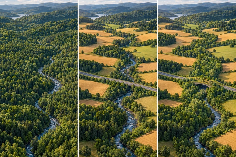 Connected habitat can permit movement; gene flow also requires successful reproduction. Conservation plans balance habitat quality, core area, representation and shared disturbance exposure.
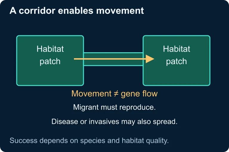 Connected habitat can permit movement; gene flow also requires successful reproduction. Conservation plans balance habitat quality, core area, representation and shared disturbance exposure.
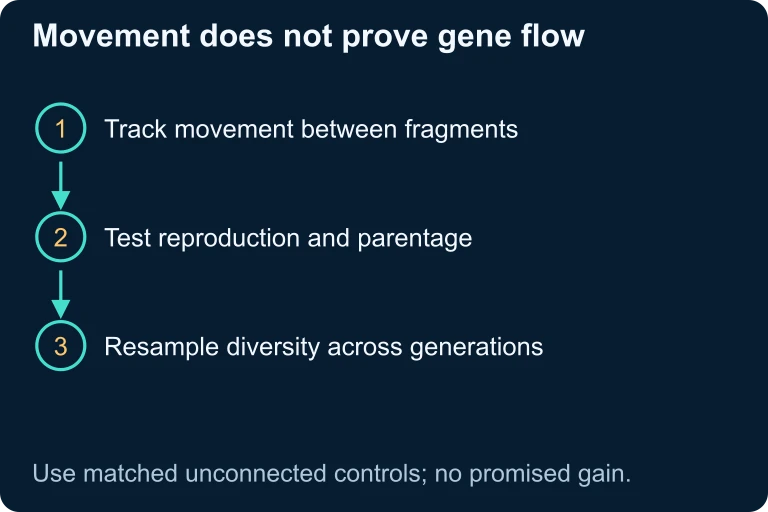 Tracking movement tests connectivity. Parentage and reproduction measurements test gene flow, and repeated genetic sampling tests changes across generations.
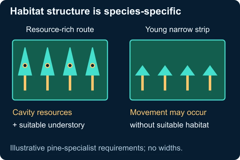 A corridor must provide the resources and habitat structure required by the focal species; movement alone does not establish suitable breeding habitat.
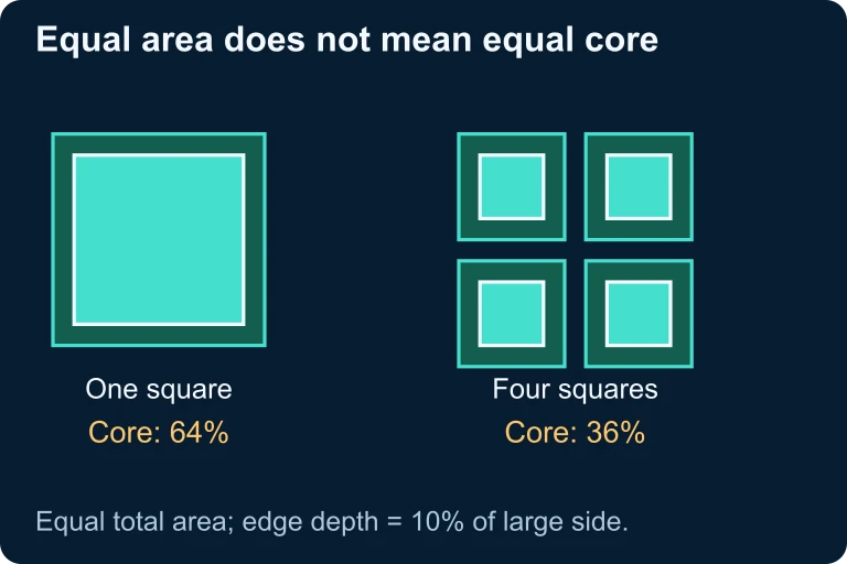 For equal total area and a fixed edge depth, one large square retains 64% core habitat while four smaller squares retain 36%.
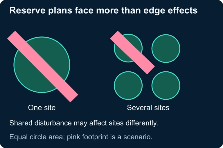 Reserve designs with equal total area can expose habitat to different shared disturbances; site arrangement is another consideration alongside core area.
SECTION 9
Practice Problems
Question 1: CONCEPTUAL
- A. Both communities have equal biodiversity because they have identical species richness.
- B. Community Y has higher biodiversity because one dominant species stabilizes the community.
- C. Community X has higher species diversity because its greater evenness produces a higher diversity index.
- D. Biodiversity cannot be compared without knowing the identities of the species present.
Show answer (C)
Question 2: BASIC CALCULATION
- A. D = 0.38
- B. D = 0.62
- C. D = 0.72
- D. D = 1.10
Show answer (B)
Question 3: INTERMEDIATE
- A. Approximately 10% of species remain
- B. Approximately 32% of species remain
- C. Approximately 56% of species remain
- D. Approximately 75% of species remain
Show answer (C)
Question 4: APPLIED
Show answer
Question 5: CRITICAL THINKING