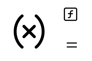
Comparing Linear, Quadratic, Polynomial, Exponential Growth - Algebra 2

SECTION 1

Historical Context & Motivation

Humans have studied patterns of growth for thousands of years. Ancient farmers tracked linear growth when planting crops in equal rows, and Greek mathematicians explored squares and cubes as they developed geometry. However, it wasn't until the development of algebra and the study of compound interest in the Renaissance that people began to notice a dramatic difference: quantities that multiply over time grow far faster than quantities that merely add. This observation sits at the heart of CCSS.F-LE.3 and is one of the most important ideas in all of mathematics.

~300 BCE • Euclid & Geometric Sequences

In Elements, Euclid explored geometric progressions—sequences where each term is a fixed multiple of the previous one—laying groundwork for the concept of exponential growth.

1614 • Napier Invents Logarithms

John Napier published tables of logarithms, giving scientists a tool to tame exponential relationships and compare vastly different scales of growth.

1683 • Jacob Bernoulli & Compound Interest

While studying compound interest, Bernoulli discovered the number e ≈ 2.718, the base of natural exponential growth, demonstrating how compounding creates explosive increases.

1798 • Malthus on Population Growth

Thomas Malthus warned that population grows exponentially while food production grows roughly linearly, predicting that exponential growth would inevitably outpace linear supply—a real-world illustration of F-LE.3.

1965 • Moore's Law

Gordon Moore observed that the number of transistors on a chip doubles roughly every two years—exponential growth in computing power that has outpaced every polynomial prediction.

The central question this lesson addresses is deceptively simple: if one quantity grows by repeated addition (like linear or polynomial functions) and another grows by repeated multiplication (like exponential functions), which one eventually dominates? As you'll see through graphs, tables, and algebraic reasoning, the answer is always the exponential—no matter how large the polynomial's degree or coefficients might be.

SECTION 2

Core Principles & Definitions

Before comparing growth types, you need clear definitions of each function family. Every function family has a distinctive structure that determines how fast its outputs increase as the input grows.

Linear Growth

A linear function has the form f(x) = mx + b. It adds a constant amount (the slope m) for every unit increase in x. Its graph is a straight line.

Quadratic Growth

A quadratic function has the form f(x) = ax² + bx + c. Its rate of change increases at a steady pace—the differences between consecutive outputs grow linearly.

Polynomial Growth

A polynomial function of degree n has the form f(x) = aₙxⁿ + … + a₁x + a₀. Higher-degree polynomials grow faster than lower-degree ones, but they still rely on repeated addition at their core.

Exponential Growth

An exponential function has the form f(x) = a · bˣ, where b > 1. It multiplies by a constant ratio for every unit increase in x, causing outputs to skyrocket.

The key distinction is between additive growth and multiplicative growth. Linear and polynomial functions grow by adding. Even x¹⁰ is just x multiplied by itself ten times—it's a fixed operation on x. An exponential function like 2ˣ, on the other hand, multiplies a base by itself x times. Because the exponent itself is the variable, the function's output doubles (or triples, etc.) with each step. This repeated multiplication eventually overwhelms any amount of repeated addition.

✦

KEY TAKEAWAY

Think of it like a race. A polynomial runner gets faster over time—maybe adding 5 mph to their speed each minute. An exponential runner doubles their speed each minute. Even if the polynomial runner starts at 1,000 mph and the exponential runner starts at 1 mph, the doubling eventually catches up and blows past every speed the polynomial runner can reach.

SECTION 3

Visual Explanation — Growth Comparison Graph

The most powerful way to understand why exponential growth dominates is to see it on a graph. The diagram below plots four functions—linear, quadratic, cubic, and exponential—on the same axes. Pay close attention to where the curves intersect and how the exponential function behaves after those crossover points.

All four functions start near each other for small values of x. The green exponential curve (2ˣ) stays below the others early on but rockets past every other function. The yellow dot marks the crossover point where the exponential surpasses the cubic, after which it never falls behind again.

Notice something important in the graph: the exponential curve 2ˣ actually starts out as the slowest function. At x = 5, the linear function 20x already equals 100, while 2⁵ is only 32. But by x = 10, 2¹⁰ = 1,024, which towers over 20(10) = 200. The exponential function doesn't need to start fast—it just needs time. Given enough runway, it will always win.

SECTION 4

Mathematical Framework

To compare growth rates formally, we examine how each function family behaves as x increases. The defining equations reveal why exponential functions eventually dominate.

LINEAR FUNCTION

f(x) = mx + b

m = constant rate of change (slope); b = y-intercept. Output increases by a fixed amount m for each unit increase in x.

POLYNOMIAL FUNCTION (DEGREE n)

f(x) = aₙxⁿ + aₙ₋₁xⁿ⁻¹ + … + a₁x + a₀

The highest-power term aₙxⁿ dominates for large x. Growth depends on the degree n: doubling x multiplies the dominant term by 2ⁿ.

EXPONENTIAL FUNCTION

g(x) = a · bˣ, where b > 1

a = initial value; b = constant growth factor. Each unit increase in x multiplies the output by b. The variable is in the exponent, not the base.

Here is the critical insight. Consider the ratio of consecutive outputs for each function type as x increases by 1:

GROWTH RATIO COMPARISON

Linear: f(x+1)/f(x) → 1 | Polynomial: f(x+1)/f(x) → 1 | Exponential: g(x+1)/g(x) = b

For linear and polynomial functions, the ratio of consecutive outputs approaches 1 as x grows large—each new output is only slightly larger than the previous one in percentage terms. For an exponential function, the ratio is always exactly b, a constant greater than 1. This constant percentage growth is what makes exponential functions unstoppable.

To put it simply: a polynomial function of degree n grows like x raised to a fixed power. An exponential function grows like a fixed base raised to x. When x is large, having x in the exponent always beats having x in the base. For any polynomial xⁿ and any exponential bˣ (with b > 1), there exists some value of x beyond which bˣ > xⁿ for all larger x.

SECTION 5

Detailed Breakdown — Comparing with Tables

Tables offer another powerful way to observe the crossover. By computing outputs for several values of x, you can see exactly when the exponential overtakes the others. Study the table below carefully and watch for the moment 2ˣ surpasses each competitor.

x	20x (Linear)	x² (Quadratic)	x³ (Cubic)	2ˣ (Exponential)
1	20	1	1	2
2	40	4	8	4
3	60	9	27	8
5	100	25	125	32
8	160	64	512	256
10	200	100	1,000	1,024
15	300	225	3,375	32,768
20	400	400	8,000	1,048,576
30	600	900	27,000	1,073,741,824

Side-by-side output comparison as x increases

At x = 5, the cubic function x³ = 125 is nearly four times larger than 2⁵ = 32. But by x = 10, the exponential 2¹⁰ = 1,024 has already surpassed the cubic's 1,000. By x = 20, the exponential has exploded to over one million while the cubic sits at only 8,000. And at x = 30, the exponential exceeds one billion—more than 39,000 times the cubic's value. This pattern only becomes more extreme as x continues to grow.

Left panel: the linear function f(x) = 3x has constant first differences of 3, while its output ratios shrink toward 1. Right panel: the exponential g(x) = 3ˣ has constant ratios of 3, while its differences grow explosively. This is the fundamental distinction between additive and multiplicative growth.

💡

How to Spot the Difference in a Table

If the differences between consecutive outputs are constant, the function is linear. If the second differences are constant, it's quadratic. If the ratios of consecutive outputs are constant, it's exponential. This is a quick diagnostic you can use on any data table.

SECTION 6

Worked Example — Finding the Crossover

Let's work through a complete problem. Suppose you're comparing the polynomial function f(x) = 5x³ with the exponential function g(x) = 3ˣ. Your task is to determine when the exponential overtakes the polynomial.

When Does 3ˣ Surpass 5x³?

1
Step 1 — Set Up a Comparison Table

Calculate both f(x) = 5x³ and g(x) = 3ˣ for several values of x. Start with small values and increase until you see the exponential overtake the polynomial.
2
Step 2 — Compute Values for Small x

At x = 1: f(1) = 5(1)³ = 5, g(1) = 3¹ = 3. At x = 5: f(5) = 5(125) = 625, g(5) = 3⁵ = 243. At x = 8: f(8) = 5(512) = 2,560, g(8) = 3⁸ = 6,561.

At x = 8, the exponential (6,561) has already surpassed the polynomial (2,560).
3
Step 3 — Narrow the Crossover

At x = 6: f(6) = 5(216) = 1,080 and g(6) = 3⁶ = 729. The polynomial is still ahead. At x = 7: f(7) = 5(343) = 1,715 and g(7) = 3⁷ = 2,187. The exponential has overtaken the polynomial.

The crossover occurs between x = 6 and x = 7.
4
Step 4 — Verify the Trend Continues

At x = 10: f(10) = 5(1,000) = 5,000 and g(10) = 3¹⁰ = 59,049. At x = 15: f(15) = 5(3,375) = 16,875 and g(15) = 3¹⁵ = 14,348,907. The gap grows enormously. Once the exponential passes the polynomial, it never falls behind again.

3ˣ permanently exceeds 5x³ for all x ≥ 7.
5
Step 5 — Interpret the Result

Even though the polynomial had a head start (it was larger for x = 1 through 6), the exponential's constant multiplication factor of 3 eventually overwhelmed the cubic's additive growth. This confirms CCSS.F-LE.3: the exponential always wins in the long run.

SECTION 7

Strengths & Limitations of Each Growth Model

Each function type is useful for modeling different real-world situations. The key is understanding which model fits the scenario and recognizing that no polynomial model is appropriate for truly exponential phenomena over the long term.

Function Type	Best Used When…	Limitations
Linear (mx + b)	A quantity increases or decreases at a constant rate—hourly wages, distance at constant speed, simple depreciation.	Cannot model accelerating or decelerating growth. Oversimplifies many real phenomena over long time spans.
Quadratic (ax² + bx + c)	Projectile motion, area calculations, situations where the rate of change itself changes at a constant rate.	Eventually dominated by exponentials; parabolas can turn downward, which may not match the scenario.
Polynomial (aₙxⁿ + …)	Complex curves, approximations of short-term trends, engineering design curves, volume formulas.	Higher degree ≠ faster than exponential; all polynomials are eventually surpassed. Harder to interpret as degree increases.
Exponential (a · bˣ)	Population growth, compound interest, radioactive decay, viral spread, Moore's Law—any scenario with a constant percentage change.	Unrealistic for unlimited time—real systems face constraints (resources, space). Often transitions to logistic growth.

When to use each growth model

✦

KEY TAKEAWAY

Exponential growth is the most powerful pattern for large x values, but it's not always the best model. A car traveling at a steady 60 mph is perfectly modeled by a linear function. The lesson of F-LE.3 isn't that 'exponential is always better'—it's that when comparing a polynomial and an exponential over the long run, the exponential always wins eventually.

SECTION 8

Connections to Advanced Theory

The idea that exponential functions eventually dominate polynomials is just the beginning of a hierarchy of growth rates studied in higher mathematics and computer science. Understanding this hierarchy prepares you for more advanced coursework.

Concept in This Lesson	Advanced Extension
Exponential eventually exceeds any polynomial	In calculus, this is proven rigorously using limits: lim(x→∞) xⁿ / bˣ = 0 for any n and any b > 1.
Comparing growth rates using tables	In computer science, Big-O notation classifies algorithms by growth rate: O(n), O(n²), O(2ⁿ). Exponential algorithms are considered impractical for large inputs.
Constant ratio characterizes exponential functions	Differential equations formalize this: if dy/dx = ky, then y = Ceᵏˣ. The rate of change being proportional to the function's value is the hallmark of exponential behavior.
Real-world exponential growth (populations, interest)	Logistic growth models (studied in AP courses) show that exponential growth transitions to a bounded curve when resources are limited: y = L / (1 + e⁻ᵏ⁽ˣ⁻ˣ⁰⁾).

From Algebra 2 to calculus and computer science

There is even a growth family faster than exponentials: factorials (n!). Just as exponentials dominate polynomials, factorials dominate exponentials. The growth-rate hierarchy goes: logarithmic < polynomial < exponential < factorial. Mastering the polynomial-versus-exponential comparison in this lesson gives you the foundational reasoning you'll need for all of these more advanced ideas.

SECTION 9

Practice Problems

Question 1: CONCEPTUAL

Explain in your own words why an exponential function like 2ˣ will eventually surpass a polynomial function like x¹⁰, even though x¹⁰ grows much faster for small values of x.

Show answer

A polynomial function like x¹⁰ grows by adding larger and larger amounts, but its percentage growth rate decreases as x increases. The ratio x¹⁰/(x−1)¹⁰ approaches 1 as x gets very large. In contrast, 2ˣ maintains a constant ratio of 2 between consecutive outputs—each value is always double the previous one. Because a fixed percentage increase (100% per step) eventually overwhelms any decreasing percentage increase, 2ˣ must eventually surpass x¹⁰. It may take a very large value of x for the crossover to happen, but it is mathematically guaranteed.

Question 2: BASIC CALCULATION

Compare f(x) = 10x and g(x) = 2ˣ by computing both values at x = 1, 5, 10, and 20. At which value of x does 2ˣ first exceed 10x?

Show answer

At x = 1: f(1) = 10, g(1) = 2. At x = 5: f(5) = 50, g(5) = 32. At x = 10: f(10) = 100, g(10) = 1,024. So 2ˣ first exceeds 10x at x = 10 (among the given values). Checking between: at x = 7, f(7) = 70 and g(7) = 128, so the crossover actually occurs between x = 6 (f = 60, g = 64) and x = 7. This confirms that even a modest exponential base of 2 overtakes a linear function relatively quickly.

Question 3: INTERMEDIATE

You are given three functions: h(x) = 100x², p(x) = x⁴, and q(x) = 1.5ˣ. Build a table for x = 10, 20, 50, and 100. Determine the order of dominance (smallest to largest) at x = 100 and explain why.

Show answer

At x = 10: h = 10,000; p = 10,000; q ≈ 57.67. At x = 20: h = 40,000; p = 160,000; q ≈ 3,325.26. At x = 50: h = 250,000; p = 6,250,000; q ≈ 637,621,500. At x = 100: h = 1,000,000; p = 100,000,000; q = 1.5¹⁰⁰ ≈ 4.06 × 10¹⁷. The order from smallest to largest at x = 100 is h(x) < p(x) < q(x). Even though 1.5 seems like a small base and the polynomial p(x) = x⁴ has a high degree with no small coefficient, the exponential 1.5ˣ crushes both by x = 100. This illustrates that any base greater than 1 will eventually dominate any polynomial, regardless of degree or leading coefficient.

Question 4: APPLIED

A city's population grows exponentially at 3% per year, modeled by P(t) = 50,000 × 1.03ᵗ (where t is years). A city planner estimates infrastructure capacity grows as C(t) = 50,000 + 200t² (a quadratic model). After how many years will the population first exceed the infrastructure capacity? What does this mean for the city?

Show answer

At t = 0, both equal 50,000. Testing values: at t = 20, P(20) = 50,000 × 1.03²⁰ ≈ 90,306 and C(20) = 50,000 + 200(400) = 130,000; capacity leads. At t = 50, P(50) ≈ 50,000 × 4.384 ≈ 219,188 and C(50) = 50,000 + 200(2,500) = 550,000; capacity still leads. At t = 100, P(100) ≈ 50,000 × 19.219 ≈ 960,923 and C(100) = 50,000 + 200(10,000) = 2,050,000; capacity still leads. At t = 150, P(150) ≈ 50,000 × 84.25 ≈ 4,212,364 and C(150) = 50,000 + 200(22,500) = 4,550,000; close. At t = 155, P ≈ 4,886,837 and C = 4,855,000. The population first exceeds capacity around t ≈ 155 years. This means the city must plan for the inevitable: even though quadratic infrastructure investment seems aggressive, exponential population growth will eventually outpace it.

Question 5: CRITICAL THINKING

A classmate claims: 'I found a polynomial that beats 2ˣ for all positive values of x. My function is f(x) = x²⁰.' Is your classmate correct? Construct an argument using the core principle of this lesson, and estimate (without a calculator) roughly how large x must be before 2ˣ overtakes x²⁰.

Show answer

The classmate is incorrect about 'all positive values.' While x²⁰ will indeed exceed 2ˣ for a very large range of x values, the fundamental principle of F-LE.3 guarantees that 2ˣ must eventually surpass x²⁰. To estimate the crossover, consider that 2ˣ doubles every step, while x²⁰ has a growth ratio of ((x+1)/x)²⁰ ≈ (1 + 20/x) for large x. When x is very large, this ratio approaches 1 + 20/x, which approaches 1. Meanwhile, 2ˣ's ratio is always 2. Once x is large enough that the polynomial's percentage growth per step drops below the exponential's 100% growth per step, the exponential begins closing the gap. A rough estimate: 2ˣ = x²⁰ when x·log(2) = 20·log(x). Trying x = 100: 100 × 0.301 = 30.1 vs. 20 × 2 = 40. Trying x = 200: 200 × 0.301 = 60.2 vs. 20 × 2.301 = 46.02. So the crossover is roughly between x = 100 and x = 200. The classmate's function wins for a long time, but not forever.

SUMMARY

Lesson Summary

Summary

This lesson explored the central claim of CCSS.F-LE.3: a quantity increasing exponentially will eventually exceed a quantity increasing linearly, quadratically, or as any polynomial function. The fundamental reason is that polynomial functions grow through repeated addition (their output ratios shrink toward 1), while exponential functions grow through repeated multiplication (their output ratio stays constant and greater than 1).

Using graphs, you saw the exponential curve start slowly and then rocket past all polynomial curves. Using tables, you confirmed that exponential outputs eventually dwarf polynomial outputs by orders of magnitude. You also learned to distinguish growth types by examining constant differences (linear), constant second differences (quadratic), and constant ratios (exponential). This concept connects forward to limits in calculus, Big-O notation in computer science, and real-world modeling of populations, finance, and technology.