Average Rate of Change - Algebra 1

Section 1

Where Did This Idea Come From?

Humans have always wanted to describe how quickly things change. Whether ancient astronomers tracked planets sliding across the night sky or merchants calculated how fast profits grew, the idea of comparing a change in output to a change in input has been around for thousands of years. The average rate of change is the formal algebraic version of that same everyday question: "How much did something change, and over what interval did it happen?"

~300 BCE • Ancient Greece

Greek mathematicians like Archimedes studied areas under curves and rates of motion. They didn't have algebra yet, but they used geometric reasoning to compare distances traveled over spans of time — an early form of rate-of-change thinking.

1300s–1400s • Medieval Scholars

At Oxford, Nicolas Oresme drew some of the first graphs of changing quantities (like speed vs. time). His work showed that you could visualize change as the slope of a line segment, setting the stage for the algebra we use today.

1600s • Galileo & Descartes

Galileo used tables and ratios to describe how falling objects speed up. Around the same time, René Descartes invented the coordinate plane, giving us the x-y framework we now use to plot functions and calculate slopes.

Late 1600s • Newton & Leibniz

Isaac Newton and Gottfried Leibniz independently invented calculus. The average rate of change became the stepping stone to the instantaneous rate of change (the derivative), one of the most powerful tools in all of mathematics.

Today • Algebra 1 & Beyond

Average rate of change is now a core algebra standard. It appears in science classes when you study velocity, in economics when you study growth, and in data analysis whenever you look at trends between two data points.

The big question this concept addresses is simple but powerful: if a function changes between two input values, how fast does it change on average across that interval? The formula gives you a single number that captures the overall trend — even if the function wiggles along the way.

Section 2

Core Principles & Definitions

Before you calculate anything, you need to understand four foundational ideas. Each one builds on your existing knowledge of functions and coordinate graphs.

Rate of Change = Slope

The average rate of change of a function over an interval is the same calculation as the slope of the line connecting two points on the graph. If you can find slope, you can find average rate of change.

Two Points Define the Interval

You always need two input values (x-values) to define an interval. The function's outputs at those two inputs give you everything you need for the calculation.

It Describes the "Big Picture"

Average rate of change ignores the bumps in the middle. It only compares the starting output to the ending output, giving you the overall trend across the whole interval.

Units Tell the Story

The rate is always "output units per input unit." For example, if y is dollars and x is hours, the average rate of change is dollars per hour. Units make the number meaningful.

✦

✦ Key Takeaway

Think of average rate of change like a road trip. Suppose you drive 150 miles in 3 hours. You probably sped up, slowed down, and maybe stopped for gas, but your average speed was 150 ÷ 3 = 50 miles per hour. That single number summarizes the whole trip. Average rate of change does the same thing for any function — it tells you the overall "speed" at which the output changes across an interval, even if the function isn't changing at a constant pace.

Section 3

Seeing It on a Graph

A picture makes this concept click. Below is a graph of a function f(x) with a curved shape. The two highlighted points sit on the curve at x = 1 and x = 5. The straight dashed line connecting them is called a secant line. The slope of that secant line is the average rate of change over the interval [1, 5].

Graph of f(x) = 0.5x² + 0.5x + 1 with a secant line from (1, 2) to (5, 10) showing Δy = 8 and Δx = 4.

Notice a few things in the diagram. The curved function rises steeply in some places and flattens in others, but the secant line draws a straight path from the starting point (1, 2) to the ending point (5, 10). The vertical change (Δy = 8) divided by the horizontal change (Δx = 4) gives the average rate of change: 8 ÷ 4 = 2. That means, on average, the function's output increased by 2 units for every 1 unit increase in x across that interval.

Section 4

The Formula & How to Use It

The average rate of change of a function f over the interval from x = a to x = b is calculated with a formula you already know in disguise — it's the slope formula, just written in function notation.

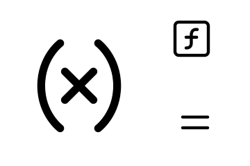
Average Rate of Change Formula

Average Rate of Change = [ f(b) − f(a) ] / ( b − a )

f(b) = function output at the end of the interval | f(a) = output at the start | b − a = length of the interval

If you've seen the slope formula m = (y₂ − y₁) / (x₂ − x₁), this is the same idea. Replace y₂ with f(b), replace y₁ with f(a), and the x-values become b and a. The numerator is the total change in the output (sometimes written Δy or Δf), and the denominator is the total change in the input (Δx).

Slope Notation (Equivalent)

m = Δy / Δx = ( y₂ − y₁ ) / ( x₂ − x₁ )

This is the same calculation — just different notation.

Here's the step-by-step process to find the average rate of change every time:

💡

Step-by-Step Method

Step 1 — Identify the interval. You need two x-values: a (start) and b (end).

Step 1 — Identify the interval. You need two x-values: a (start) and b (end).
Step 2 — Find the function's output at each endpoint. If given a formula, plug in a and b. If given a table, look up the y-values.
Step 3 — Subtract the outputs: f(b) − f(a). This is the change in y.
Step 4 — Subtract the inputs: b − a. This is the change in x.
Step 5 — Divide: (f(b) − f(a)) / (b − a). This quotient is the average rate of change.
Step 6 — Interpret. Explain what the number means using the context and units of the problem.

Sign Matters

Positive → output increases | Negative → output decreases | Zero → no net change

The sign of the average rate of change tells you whether the function is going up or down (on average) across the interval.

Section 5

Working From a Table vs. a Formula

You'll encounter average rate of change in two main formats: functions given as equations and functions given as tables of values. The process is the same either way, but the way you find f(a) and f(b) differs.

Two paths to the same formula: from an equation (left) or from a table (right).

Example With a Table

Suppose you're given the following table and asked to find the average rate of change from x = 1 to x = 4.

x	f(x)
0	5
1	8
2	13
3	20
4	29
5	40

From the table, f(1) = 8 and f(4) = 29. So the average rate of change is (29 − 8) / (4 − 1) = 21 / 3 = 7. The output grew by an average of 7 units per 1 unit of x over that interval. Notice that you don't need to worry about what happened at x = 2 or x = 3 — only the endpoints matter.

Example With a Formula

If g(x) = 2x² − 1, find the average rate of change on [1, 3]. First, evaluate: g(1) = 2(1)² − 1 = 1 and g(3) = 2(3)² − 1 = 17. Then divide: (17 − 1) / (3 − 1) = 16 / 2 = 8. The function's output increased at an average rate of 8 units per unit of x.

Section 6

Full Worked Example

Let's work through a real-world problem from start to finish, showing every detail.

Plant Growth — Average Rate of Change

1
Problem

A plant's height (in centimeters) is modeled by the function h(t) = t² + 2t + 5, where t is the number of weeks after planting. Find and interpret the average rate of change of the plant's height from week 1 to week 4.
2
Step 1 — Identify the Interval

The interval is from t = 1 to t = 4. So a = 1 and b = 4.
3
Step 2 — Find the Output at Each Endpoint

Evaluate h(1):

h(1) = (1)² + 2(1) + 5 = 1 + 2 + 5 = 8
4
Step 2 (continued)

Evaluate h(4):

h(4) = (4)² + 2(4) + 5 = 16 + 8 + 5 = 29
5
Step 3 — Subtract the Outputs (Numerator)

Calculate the change in output:

h(4) − h(1) = 29 − 8 = 21
6
Step 4 — Subtract the Inputs (Denominator)

Calculate the change in input:

4 − 1 = 3
7
Step 5 — Divide

Compute the average rate of change:

Average Rate of Change = 21 / 3 = 7
8
Step 6 — Interpret

The average rate of change is 7 centimeters per week. This means that between week 1 and week 4, the plant grew an average of 7 cm each week. The plant might have grown faster in some weeks and slower in others, but 7 cm/week captures the overall trend.

Section 7

Strengths, Limitations & Comparisons

Average rate of change is incredibly useful, but it's important to know what it can and can't tell you. Let's compare it with a few related ideas.

Feature	Average Rate of Change	Actual Rate at a Single Point
What it measures	Overall change across an interval	Speed of change at one exact moment
Data needed	Two points (or two function values)	Requires calculus (derivatives)
Graph interpretation	Slope of the secant line	Slope of the tangent line
For linear functions	Same everywhere — the constant slope	Same everywhere — identical result
For non-linear functions	Depends on which interval you choose	Changes from point to point
Accessible in Algebra 1?	Yes ✓	Not yet — needs calculus

Strengths: Average rate of change is simple to compute, requires no calculus, and gives a clear summary of how a function behaves across any interval you pick. It works for functions given as formulas, tables, or even graphs (where you read coordinates).

Limitations: It hides what happens inside the interval. A function could rise sharply and then fall, yet the average rate of change might still be positive if the endpoint is higher than the start. Two very different functions could have the same average rate of change over the same interval if they start and end at the same values.

✦

✦ Key Takeaway

Average rate of change is like checking your bank balance on Monday and again on Friday. If you had $50 on Monday and $90 on Friday, your money grew by an average of $10 per day. But that doesn't mean you earned exactly $10 each day — maybe you received $60 on Wednesday and spent $20 on Thursday. The average captures the net trend, not the day-by-day details. When you need more detail, you'll shrink the interval or, eventually, use calculus.

Section 8

Connection to Advanced Ideas

If you continue into Pre-Calculus and Calculus, the average rate of change becomes the launching pad for one of the most important concepts in mathematics: the derivative. Here's how the two connect.

When you calculate the average rate of change over the interval [a, b], you're measuring the secant line's slope. Now imagine sliding point b closer and closer to a. The interval shrinks, and the secant line begins to rotate toward the curve. In the limit — when the two points are "infinitely close" — the secant line becomes a tangent line, and its slope is the instantaneous rate of change, also called the derivative. You don't need to master this yet, but it's valuable to know that everything you're learning here leads directly to that powerful idea.

Concept	Average Rate of Change (Algebra 1)	Derivative (Calculus)
Formula	`[f(b) − f(a)] / (b − a)`	`lim (h→0) [f(a+h) − f(a)] / h`
Interval size	Finite (b − a > 0)	Approaches zero
Result	One slope for the whole interval	A slope at a single point
Graphically	Slope of secant line	Slope of tangent line

For now, focus on mastering the average rate of change. It builds your fluency with function notation, strengthens your understanding of slope, and gives you a conceptual head start for the mathematics ahead.

Section 9

Practice Problems

Try each problem before revealing the answer. The difficulty increases as you go.

Question 1: Conceptual

In your own words, explain why the average rate of change of a linear function is the same no matter which interval you choose. What property of linear functions makes this true?

Show answer

A linear function has the form f(x) = mx + b, where the slope m is constant. Because the function rises (or falls) at the same steady rate everywhere, the ratio of change in y to change in x is always m, regardless of which two x-values you pick. No matter how wide or narrow the interval, the secant line has the same slope as the function itself — they are the same line. This is what makes linear functions special: constant rate of change.

Question 2: Basic Calculation

Use the table below to find the average rate of change of f(x) from x = 2 to x = 6. | x | f(x) | |---|------| | 0 | 3 | | 2 | 11 | | 4 | 27 | | 6 | 51 | | 8 | 83 |

Show answer

From the table, f(2) = 11 and f(6) = 51. Apply the formula: Average Rate of Change = (51 − 11) / (6 − 2) = 40 / 4 = 10. The function's output increased by an average of 10 units per unit of x over the interval [2, 6].

Question 3: Intermediate

Let f(x) = −x² + 6x. Find the average rate of change on the interval [1, 5]. Is the result positive or negative, and what does the sign tell you?

Show answer

Evaluate the function at each endpoint: f(1) = −(1)² + 6(1) = −1 + 6 = 5 and f(5) = −(5)² + 6(5) = −25 + 30 = 5. Average Rate of Change = (5 − 5) / (5 − 1) = 0 / 4 = 0. The average rate of change is zero. This means the function's output at x = 5 is the same as at x = 1, so there is no net change over that interval. The function goes up in the middle and comes back down, but the starting and ending heights are equal. A rate of zero does not mean nothing happened — it means the increases and decreases canceled out.

Question 4: Applied / Multi-Step

A car's distance from home (in miles) is recorded in the table below. Find the average rate of change from t = 0.5 hours to t = 2 hours. Then explain what this rate means in real-world terms, including units. | Time t (hours) | Distance d(t) (miles) | |---|---| | 0 | 0 | | 0.5 | 18 | | 1 | 40 | | 1.5 | 55 | | 2 | 78 | | 2.5 | 78 |

Show answer

From the table: d(0.5) = 18 miles and d(2) = 78 miles. Average Rate of Change = (78 − 18) / (2 − 0.5) = 60 / 1.5 = 40. The average rate of change is 40 miles per hour. This means that between 0.5 hours and 2 hours after leaving home, the car traveled at an average speed of 40 mph. The car's actual speed at any moment may have been higher or lower, but 40 mph summarizes the overall pace across that 1.5-hour window.

Question 5: Challenge / Synthesis

For the function f(x) = x² − 4x + 7, the average rate of change over the interval [2, k] equals 5. Find the value of k. (Hint: set up the average rate of change formula equal to 5 and solve for k.)

Show answer

First, find f(2) = (2)² − 4(2) + 7 = 4 − 8 + 7 = 3. Next, find f(k) in terms of k: f(k) = k² − 4k + 7. Set up the average rate of change equal to 5: [f(k) − f(2)] / (k − 2) = 5 → [(k² − 4k + 7) − 3] / (k − 2) = 5 → (k² − 4k + 4) / (k − 2) = 5. Notice the numerator factors: k² − 4k + 4 = (k − 2)². So: (k − 2)² / (k − 2) = k − 2 = 5. Therefore k = 7. Check: f(7) = 49 − 28 + 7 = 28. Average rate of change = (28 − 3) / (7 − 2) = 25 / 5 = 5 ✓. This problem shows how average rate of change connects algebra skills like factoring to function analysis — a great preview of ideas you'll see in Algebra 2 and beyond.

Summary

Putting It All Together

Summary

The average rate of change of a function measures how quickly the output changes, on average, across a specified interval. It is calculated with the formula [f(b) − f(a)] / (b − a), which is identical to the slope of the secant line connecting the two corresponding points on the graph. A positive result means the function's output increased overall; a negative result means it decreased; and a result of zero means the output ended where it started, even if it changed in the middle.

You can apply this formula whether the function is given as an equation (plug in the endpoints) or as a table (read off the values directly). Always finish by interpreting your answer in context, including units. This concept is the algebraic foundation for the derivative in calculus, making it one of the most important ideas in your math education so far.